Daniel
OPERATING SYSTEMS
Intro
2 Introduction
The primary way the OS does this is through a general technique that we call virtualization. That is, the OS takes a physical resource(such as the processor, or memory, or a disk) and transfroms it into a more general, powerful, and easy-to-use virtual form of itself. Thus, we sometimes refer to the operating system as a virtual machine.
The OS provides some interface(APIS) that you can call. A typical OS, in fact, exports a few hundred system calls that are available to applications. The OS provides a standard library to applications.
2.1 Virtualizing The CPU
Turning a single CPU(or a small set of them) into a seemingly infinite number of CPUs and thus allowing many programs to seemingly run at once is what we call virtualizing the CPU.
2.2 Virtualizing Memory
Each process accesses its own private virtual address space(sometimes just called its address space), which the OS somehow maps onto the physical memory of the machine.
2.3 Concurrency
We use concurrency to refer a host of problems that arise, and must be addressed, when working on many things at once in the same program.
2.4 Persistence
The software in the operating system that usually manages the disk is called the file system; it is thus responsible for storing any files the user creates in a reliable and efficient manner on the disk of the system.
Unlike the abstraction provided by the OS for the CPU and memory, the OS does not create a private, virtualized disk for each application. Rather, it is assumed that often times, users will want to share information that is in files.
Virutalization
4 Processes
4.3 Process Creation: A little More Detail
The first thing that the OS must do to run a program is to load its code and any static data into memory, into the address space of the proces.
A process can be in one of three status:
- Running: In the running state, a process is running on a processor. This means it is executing instructions.
- Ready: In the ready state, a process is ready to run but for some reason the OS has chosen not to run it at this given moment.
- Blocked: In the blocked state, a process has performed some kind of operation that makes it not ready to run until some other event take place. A common example: when a process initiates an I/O request to a disk, it becomes blocked and thus some other process can use the processor.
Being moved from ready to running means the process has been scheduled; being moved from running to ready means the process has been descheduled. Once a process has become blocked(e.g., by initating an I/O operation), the OS will keep it as such util some event occurs(e.g., I/O completion); at that point, the process moves to the ready state again(and potentially immediately to running again, if the OS so decides).
5 Process API
5.3 Finally, The exec() System call
p3.c
#include <stdio.h>
#include <stdlib.h>
#include <unistd.h>
#include <string.h>
#include <sys/wait.h>

int
main(int argc, char *argv[])
{
    printf("hello world (pid:%d)\n", (int) getpid());
    int rc = fork();
    if (rc < 0) {
        // fork failed; exit
        fprintf(stderr, "fork failed\n");
        exit(1);
    } else if (rc == 0) {
        // child (new process)
        printf("hello, I am child (pid:%d)\n", (int) getpid());
        char *myargs[3];
        myargs[0] = strdup("wc");   // program: "wc" (word count)
        myargs[1] = strdup("p3.c"); // argument: file to count
        myargs[2] = NULL;           // marks end of array
        execvp(myargs[0], myargs);  // runs word count
        printf("this shouldn't print out");
    } else {
        // parent goes down this path (original process)
        int wc = wait(NULL);
        printf("hello, I am parent of %d (wc:%d) (pid:%d)\n",
	       rc, wc, (int) getpid());
    }
    return 0;
}
The code above is the same as “ws p3.c”
5.4 Why? Motivating The API
The Shell shows you a prompt and then waits for you to type something into it. You then type a command into it; in most cases, the shell then figures out where in the file system the executable resides, calls fork() to create a new child process to run the command, calls some variant of exec() to run the command, and then waits for the command to complete by calling wait(). When the child completes, the shell returns from wait() and prints out a prompt again, ready for your next command.
p4.c
#include <stdio.h>
#include <stdlib.h>
#include <unistd.h>
#include <string.h>
#include <fcntl.h>
#include <assert.h>
#include <sys/wait.h>

int
main(int argc, char *argv[])
{
    int rc = fork();
    if (rc < 0) {
        // fork failed; exit
        fprintf(stderr, "fork failed\n");
        exit(1);
    } else if (rc == 0) {
	// child: redirect standard output to a file
	close(STDOUT_FILENO);
	open("./p4.output", O_CREAT|O_WRONLY|O_TRUNC, S_IRWXU);

	// now exec "wc"...
        char *myargs[3];
        myargs[0] = strdup("wc");   // program: "wc" (word count)
        myargs[1] = strdup("p4.c"); // argument: file to count
        myargs[2] = NULL;           // marks end of array
        execvp(myargs[0], myargs);  // runs word count
    } else {
        // parent goes down this path (original process)
        int wc = wait(NULL);
	assert(wc >= 0);
    }
    return 0;
}
The code above is the same as ‘wc p4.c > p4.output’
6 Direct Execution
6.1 Basic Technique: Limited Direct Execution
Without limits on running programs, the OS wouldn’t be in control of anything and thus would be “just a library” – a very sad state of affairs for an aspiring operating system!
6.2 Problem #1: Restricted Operations
The hardware assists the OS by providing different modes of execution. In user mode, applications do not have full access to hardware resources. In kernel mode, the OS has access to the full resources of the machine.
What is the difference between Trap and Interrupt?
To execute a system call, a program must execute a special trap instruction. This instruction simultaneously jumps into the kernel and raises the privilege level to kernel mode; once in the kernel, the system can now perform whatever privileged operations are needed(if allowed), and thus do the required work for the calling process. When finished, the OS calls a special return-from-trap instruction, which, as you might expect, returns into the calling user program while simultaneously reducing the privilege level back to user mode.
There are two phases in the limited direct execution(LDE) protocol. In the first(at boot time), the kernel initializes the trap table, and the CPU remembers its location for subsequent use. The kernel does so via a priviledged instruction(all priviledged are highlighted in bold). In the second(when running a process), the kernel sets up a few things(e.g., allocating a node on the process list, allocating memory) before using a return-from-trap instruction to start the exeuction of the process; this switches the CPU to user mode and begins running the process. When the process wishes to issue a system call, it traps back into the OS, which handles it and once again returns control via a return-from-trap to the process. The process then completes its work, and returns from main(); this usually will return into some stub code which will properly exit the program(say, by calling the exit() system call, which traps into the OS). At this point, the OS cleans up and we are done.
6.3 Problem #2: Switching Between Process
A timer device can be programmed to raise an interrupt every so many milliseconds; when the interrupt is raised, the currently running process is halted, and a pre-configured interrupt handler in the OS runs. At this point, the OS has regained control of the CPU, and thus can do what it pleases: stop the current process, and start a different one.
Note that the hardware has some responsibility when an interrupt occurs, in particular to save enough of the state of the program that was running when the interrupt occurred such that a subsequent return-from-trap instruction will be able to resume the running program correctly. This set of actions is quite similar to the behavior of the hardware during an explicit system-call trap into the kernel, with various registers thus getting saved and thus easily restored by the return-from-trap instruction.
A cooperative approach: wait for system calls
The OS trusts the processes of the system to behave reasonably. Processes that run for too long are assumed to periodically give up the CPU so that the OS can decide to run some other task.
A non-cooperative approach: the OS takes control
A timer device can be programmed to raise an interrupt every so many milliseconds; when the interrupt is raised, the currently running process is halted, and a pre-configured interrupt handler in the OS runs. At this point, the OS has regained control of the CPU, and thus can do what is pleases: stop the current process, and start a different one.
A context switch is conceptually simple: all the OS has to do is save a few register values for the currently-executing process(onto its kernel stack, for example) and restore a few for the soon-to-be-executing process(from its kernel stack). By doing so, the OS thus ensures that when the return-from-trap instruction is finally executed, instead of returning to the process that was running, the system resumes execution of another process.
Process A is running and then is interrupted by the timer interrupt. The hardware saves its registers(onto its kernel stack) and enters the kernel(switch to kernel mode). In the timer interrupt handler, the OS decides to switch from running Process A to Process B. At that point, it calls the switch() routine, which carefully saves current register values(into the process structure of A), restores the registers of Process B(from its process structure entry), and then switches contexts, specifically by changing the stack pointer to use B’s kernel stack(and not A’s). Finally, the OS returns-from-trap, which restores B’s registers and starts running it. Note that there are two types of register saves/restores that happen during this protocol. The first is when the timer interrupt occurs; in this case, the user registers of the running process are implicitly saved by the hardware, using the kernel stack of that process. The second is when the OS decides to switch from A to B; in this case, the kernel registers are explicitly saved by software(i.e., the OS), but this time into memory in the process structure of the process. The latter action moves the system from running as if it just trapped into the kernel from A to as if it just trapped into the kernel from B.
7 Scheduling: Introduction
7.2 Scheduling Metrics
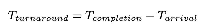
The turnaround time of a job is defined as the time at which the job completes minus the time at which the job arrived in the system.
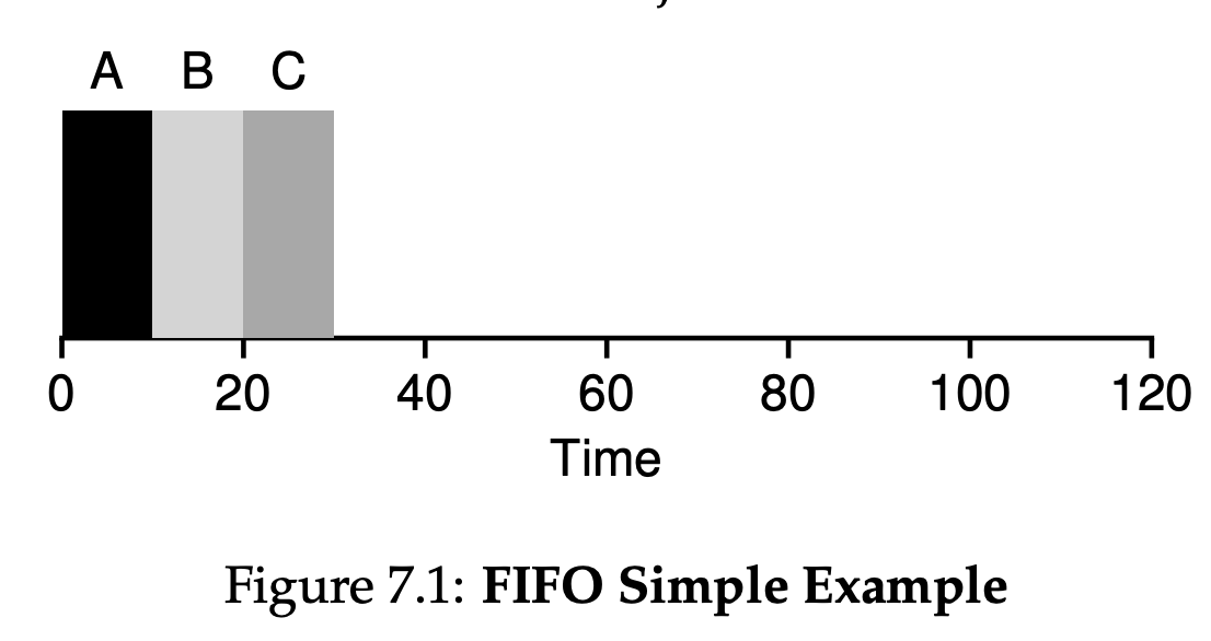
7.3 First In, First Out(FIFO)
From Figure 7.1, you can see that A finished at 10, B at 20, and C at 30. Thus, the average turnaround time for the three jobs is simply $\frac{10 + 20 + 30}{3} = 20$.
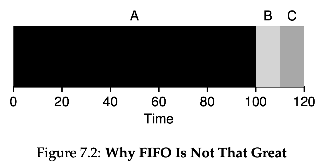
As you can see in Figure 7.2, Job A runs first for the full 100 seconds before B or C even get a chance to run. Thus, the average turnaround time for the system is high: a painful 110 seconds($\frac{100 + 110 + 120}{3} = 110$).
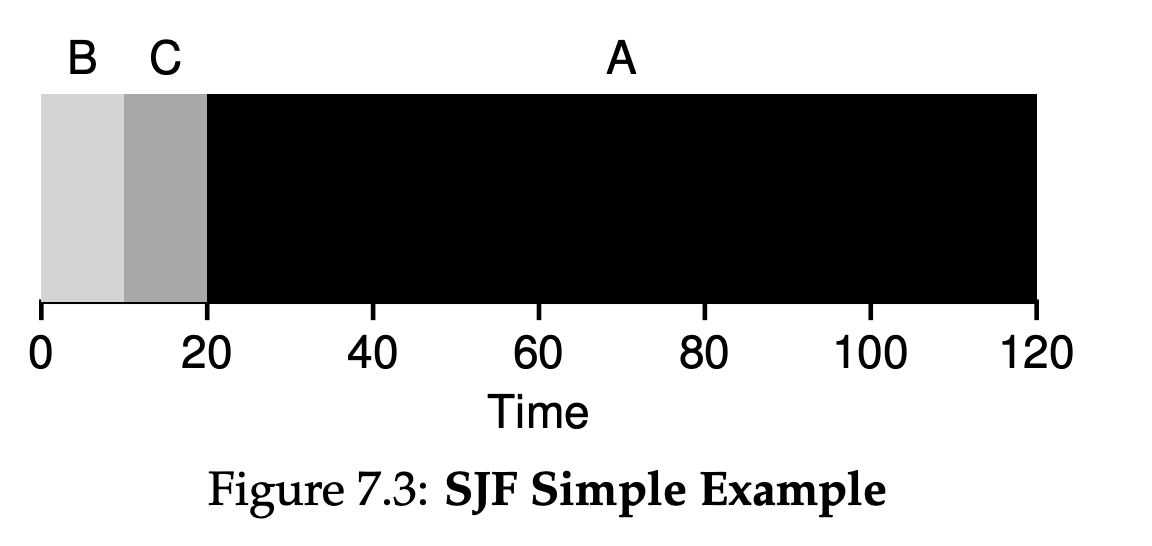
7.4 Shortest Job First(SJF)
Figure 7.3 shows the results of running A, B, and C. Hopefully the diagram make it clear why SJF performs much better with regards to average turnaround time. Simply by running B and C before A, SJF reduces average turnaround from 110 seconds to 50($\frac{10 + 20 + 120}{3} = 50$), more than a factor of two improvement.
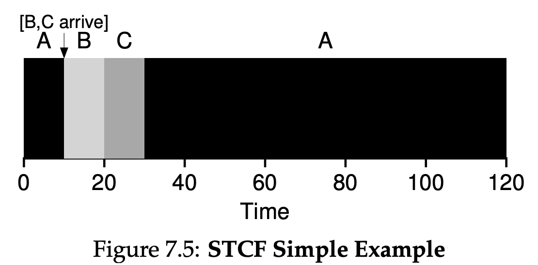
7.5 Shortest Time-to-Completion First(STCF)
Any time a new job enters the system, the STCF scheduler determines which of the remaining jobs(including the new job) has the least time left, and schedules that one. Thus, in our example, STCF would preempt A and run B and C to completion; only when they are finished would A’s remaining time be scheduled. Figure 7.5 shows an example. The result is a much-improved average turnaround time: 50 seconds($\frac{(120 - 0) + (20 - 10) + (30 - 10)}{3}$).
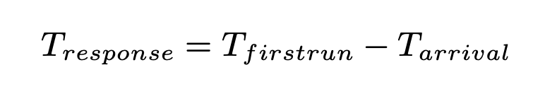
7.6 A New Metric: Response Time
We define response time as the time from when the job arrives in a system to the first time it is scheduled.
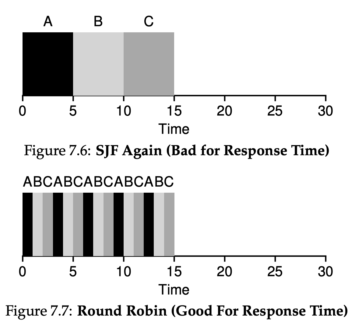
As you might be thinking, STCF and related disciplines are not particularly good for response time. If three jobs arrive at the same time, for example, the third job has to wait for the previous two jobs to run in their entirety before being scheduled just once. While great for turnaround time, this approach is quite bad for response time and interactivity. Indeed, imagine sitting at a terminal, typing, and having to wait 10 seconds to see a response from the system just because some other job got scheduled in front of yours: not too pleasant.
7.7 Round Robin
The basic idea is simple: instead of running jobs to completion, RR runs a job for a time slice(sometimes called a scheduling quantum) and then switches to the next job in the run queue. It repeatedly does so until the jobs are finished.
Assume three jobs A, B and C arrive at the same time in the system, and that they each wish to run for 5 seconds. An SJF scheduler runs each job to completion before running another. In contrast, RR with a time-slice of 1 second would cycle through the jobs quickly. The average response time of RR is: $\frac{(0 + 1 + 2)}{3} = 1$; for SJF, average response time is: $\frac{(0 + 5 + 10)}{3} = 5$.
As you can see, the length of the time slice is critical for RR. The shorter it is, the better the performance of RR under the response-time metric. However, making the time slice too short is problematic: suddenly the cost of context switching will dominate overall performance. Thus, deciding on the length of the time slice presents a trade-off to a system designer, making it long enough to amortize the cost of switching without making it so long that the system is no longer responsive.
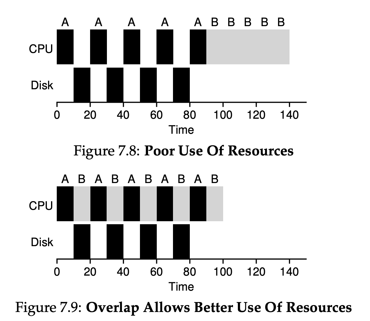
7.8 Incorporating I/O
A common approach is to treat each 10-ms sub-job of A as an independent job. Thus, when the system starts, its choice is whether to schedule a 10-ms A or a 50-ms B. With STCF, the choice is clear: choose the shorter one, in this case A. Then, when the first sub-job of A is submitted, and it preempts B and runs for 10 ms. Doing so allows for overlap, with the CPU being used by one process while waiting for the I/O of another process to complete; the system is thus better utilize.
8 Scheduling: The Multi-Level Feedback Queue
8.1 MLFQ: Basic Rules
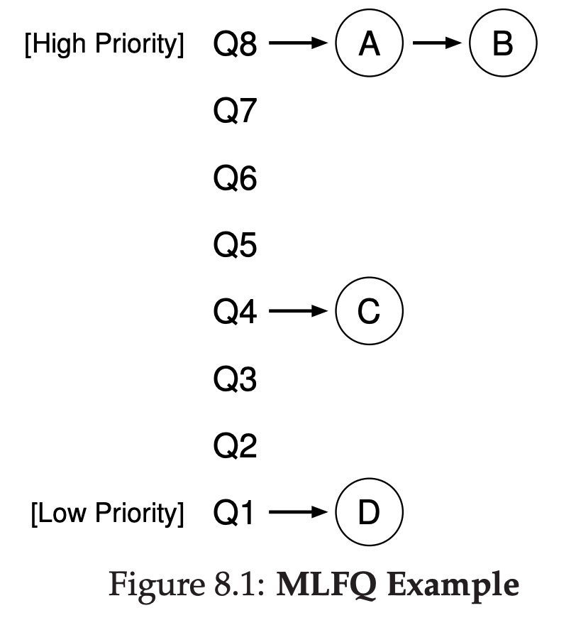
The MLFQ(Multi-level Feedback Queue) has a number of distinct queues, each assigned a different priority level. At any given time, a job that is ready to run is on a single queue. MLFQ uses priorities to decide which job should run at a given time: a job with higher priority is chosen to run. More than one job may be on a given queue, and thus have the same priority. In this case, we will just use round-robin scheduling among thoes jobs.
- Rule 1: If priority(A) > Priority(B), A runs(B doesn’t).
- Rule 2: If priority(A) = Priority(B), A & B run in RR.
The key to MLFQ scheduling therefore lies in how the scheduler sets priorities. Rather than giving a fixed priority to each job, MLFQ varies the priority of a job based on its observed behavior. If, for example, a job repeatedly relinquishes the CPU while waiting for input from the keyboard, MLFQ will keep its priority high, as this is how an interactive process might behave. If, instead, a job uses the CPU intensively for long periods of time, MLFQ will reduce its priority. In this way, MLFQ will try to learn about processes as they run, and thus use the history of the job to predict its future behavior.
8.2 Attempt #1: How To Change Priority
- Rule 3: When a job enters the system, it is placed at the hightest priority(the topmost queue).
- Rule 4a: If a job uses up an entire time slice while running, its priorityis reduced(i.e., it moves down one queue).
- Rule 4b: If a job gives up the CPU before the time slice is up, it stays at the same priority level.
8.3 Attempt #2: The Priority Boost
- Rule 5: After some time period S, move all the jobs in the system to the topmost queue.
8.4 Attempt #3: Better Accounting
Rewrite Rules 4a and 4b to the following single rule:
- Rule 4: Once a job uses up its time allotment at a given level(regardless of how many times it has given up the CPU), its priority is reduced(i.e., it moves down one queue).
8.5 Tuning MLFQ And Other Issues
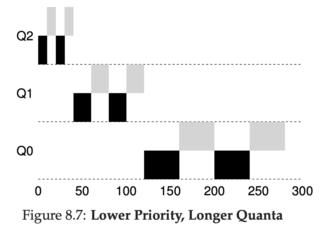
The high-priority queues are usually given short time slices; they are comprised of interactive jobs, after all, and thus quickly alternating between them makes sense. The low-priority queues, in contrast, contain long-running jobs that are CPU-bound; hence, longer time slices work well. Figure 8.7 shows an example in which two jobs run for 20ms at the highest queue(with a 10-ms time slice), 40ms in the middle(20-ms time slice), and with a 40ms time slice at the lowest.
8.6 MLFQ: Summary
It has multiple levels of queues, and uses feeback to determine the priority of a given job.
The refined set of MLFQ rules:
- Rule 1: If Priority(A) > Priority(B), A runs(B doesn’t).
- Rule 2: If Priority(A) = Priority(B), A & B run in round-robin fashion using the time slice(quantum length) of the given queue.
- Rule 3: When a job enters the system, it is placed at the highest priority(the topmost queue).
- Rule 4: Once a job uses up its time allotment at a given level(regardless of how many times it has given up the CPU), its priority is reduced(i.e., it moves down one queue).
- Rule 5: After some time period S, move all the jobs in the system to the topmost queue.
MLFQ is interesting for the following reason: instead of demanding a priori knowledge of the nature of a job, it observers the execution of a job and prioritizes it accordingly. In this way, it manages to achieve the best of both worlds: it can deliver excellent overall performance(similar to SJF/STCF) for short-running interactive jobs, and is fair and makes progress for long-running CPU-intensive workloads.
9 Scheduling: Proportional Share
Proportional-share is based around a simple concept: instead of optimizing for turnaround or response time, a scheduler might instead try to guarantee that each job obtain a certain precentage of CPU time.
9.1 Basic Concept: Tickets Represent Your Share
Underlying lottery scheduling is one very basic concept: tickets, which are used to represent the share of a resource that a process should receive. Imagine two processes, A and B, and further that A has 75 tickets while B has only 25. Thus, what we would like is for A to receive 75% of the CPU and B the remaining 25%. The longer these two jobs compete, the more likely they are to achieve the desired percentages.
9.2 Ticket Mechanisms
Lottery scheduling also provides a number of mechanisms to manipulate tickets in different and sometimes useful ways.
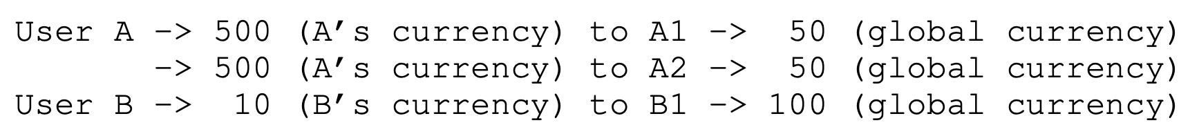
- Ticket currency allows a user with a set of tickets to allocate tickets among their own jobs in whatever currency they would like; the system then automatically converts said currency into the correct global value. For example, assume users A and B have each been given 100 tickets. User A is running two jobs, A1 and A2, and gives them each 500 tickets in A’s currency. User B is running only 1 job and gives it 10 tickets. They system converts A1’s and A2’s allocation from 500 each in A’s currency to 50 each in th global currency; similarly, B1’s 10 tickets is converted to 100 tickets. The lottery is then held over the global ticket currency to determine which job runs.
- With ticket transfer, a process can temporarily hand off its tickets to another process. This ability is especially useful in a client/server setting, where a client process sends a message to a server asking it to do some work on the client’s behalf. To speed up the work, the client can pass the tickets to the server and thus try to maximize the performance of the server while the server si handling the client’s request. When finished, the server then transfers the tickets back to the client and all is as before.
- With ticket inflation, a process can temporarily raise or lower the number of tickets it owns. Inflation can be applied in an environment where a group of processes trust one another; in such a case, if any one process knows it needs more CPU time, it can boost its ticket value as a way to reflect that need to the system, all without communicating with any other processes.
9.6 Stride Scheduling
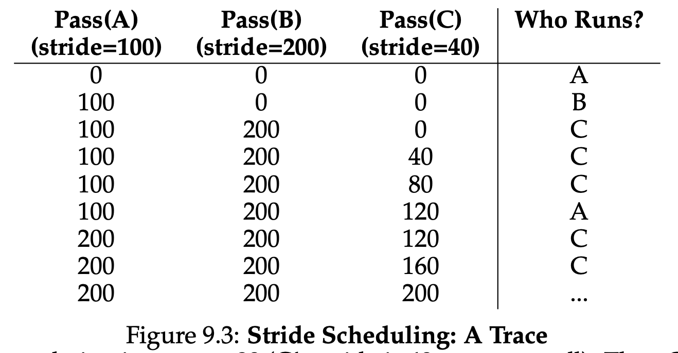
Each job in the system has a stride, which is inverse in proportion to the number of tickets it has. For example, with jobs A,B and C, with 100, 50 and 250 tickets, respectively, we can compute the stride of each by dividing some large number by the number of tickets each process has been assigned. For instance, if we divide 10000 by each of those ticket values, we obtain the following stride values for A,B and C: 100,200, and 40. We call this value the stride of each process; every time a process runs, we will increment a counter for it(called its pass value) by its stride to track its global progress. The basic idea is simple: at any given time, pick the process to run that has the lowest pass value so far; when you run a process, increment its pass counter by its stride.
9.7 The Linux Completely Fair Scheduler(CFS)
Whereas most schedulers are based around the concept of a fixed time slice, CFS operates a bit differently. Its goal is simple: to fairly divide a CPU evenly among all competing processes. It does so through a simple counting-based technique known as virtual runtime(vruntime). As each process runs, it accumulates vruntime. In the most basic case, each process’s vruntime increases at the same rate, in proportion with physical(real) time. When a scheduling decision occurs, CFS will pick the process with the lowest vruntime to run next.
CFS uses sched_latency to determine how long one process should run before considering a switch(effectively determining its time slice but in a dynamic fashion). A typical sched_latency value is 48(milliseconds); CFS divides this value by the number(n) of processes running on the CPU to determine the time slice for a process, and thus ensures that over this period of time, CFS will be completely fair.
CFS will never set the time slice of a process to less than min_granularity, which is usually set to a value like 6ms, ensureing that not too much time is spent in scheduling overhead.
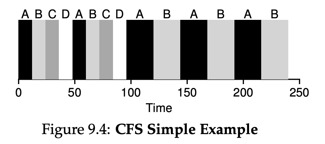
For example, if there are n = 4 processes running, CFS divides the value of sched_latency by n to arrive at a pre-process time slice of 12ms. CFS then schedules the first job and runs it until it has used 12ms of (virtual) runtime, and then checks to see if there is a job with lower vruntime to run instead. Figure 9.4 shows an example where the four jobs(A,B,C,D) each run for two time slices in this fashion; two of them(C,D) then complete, leaving just two remaining, which then each run for 24ms in round-robin fashion.
CFS also enables controls over process priority, enabling users or administrators to give some processes a higher share of the CPU. It does this not with tickets, but through a classic UNIX mechanism known as the nice level of a process. The nice parameter can be set anywhere from -20 to +19 for a process, with a default of 0. Positive nice values imply lower priority and negative values imply higher priority; when you’re too nice, you just don’t get as much(scheduling) attention, alas.
CFS is keeping processing in a red-black tree. CFS does not keep all process in this structure; rather, only running(or runnable) processes are kept therein. If a process goes to sleep(say, waiting on an I/O to complete, or for a network packet to arrive), it is removed from the tree and ketp track of elsewhere.
One problem with picking the lowest vruntime to run next arises with jobs that have gone to sleep for a long period of time. CFS handles this case by altering the vruntime of a job when it wakes up. Specifically, CFS sets the vruntime of that job to the minimum value found in the tree.
10 Multiprocessor Scheduling(Advanced)
10.1 Background: Multiprocessor Architecture
To understand the new issues surrounding multiprocessor scheduling, we have to understand a new and fundamental difference between single-CPU hardware and multi-CPU hardware. This difference centers around the use of hardware cahces, and exactly how data is shared across multiple processors.
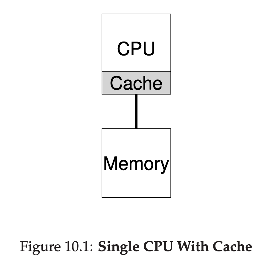
In a system with a single CPU, there are a hierarchy of hardware caches that in general help the processor run programs faster. Caches are small, fast memories that(in general) hold copies of popular data that is found in the main memory of the system. Main memory, in contrast, hold all of the data, but access to this larger memory is slower. By keeping frequently accessed data in a cache, the system can make the large, slow memory appear to be a fast one.
Caches are thus based on the notion of locality, of which there are two kinds: temporal locality and spatial locality. The idea behind temporal locality is that when a piece of data is accessed, it is likely to be accessed again in the near future; imagine variables or even instructions themeselves being accessed over and over again in a loop. The idea behind spatial locality is that if a program accesses a data item at address x, it is likely to access data items near x as well; here, think of a program streaming through an array, or instructions being executed one after the other. Because locality of these types exist in many programs, hardware systems can make good guesses about which data to put in a cache and thus work well.
Caching with multiple CPUs is much more complicated. Imagine, for example, that a program running on CPU 1 reads a data item(with value D) at address A; because the data is not in the cache on CPU 1, the system fetches it from main memory, and gets the value D. The program then modifies the value at address A, just updating its cache with the new value D’; writing the data through all the way to main memory is slow, so the system will(usually) do that later. Then assume the OS decides to stop running the program and move it to CPU 2. The program then re-reads the value at address A; there is no such data CPU 2’s cache, and thus the system fetches the value from main memory, and gets the old value D instead of the correct value D’. Oops! This general problem is called the problem of cache coherence. The basic solution is provided by the hardware: by monitoring memory accesses, hardware can ensure that basically the “right thing” happens and that the view of a single shared memory is preserved. One way to do this on a bus-based system is to use an old technique known as bus snooping; each cache pays attention to memory updates by observing the bus that connects them to main memory. When a CPU then sees an update for a data item it holds in its cache, it will notice the change and either invalidate its copy(i.e., remove it from its own cache) or update it(i.e., put the new value into its cache too). Write-back caches, as hinted as above, make this more complicated(because the write to main memory isn’t visible until later), but you can imagine how the basic scheme might work.
10.2 Don’t Forget Synchronization
When accessing shared data items or structures across CPUs, mutual exclusion primitives(such as locks) should likely be used to guarantee correctness.
Locking is not without problems, in particular with regards to performance. Specifially, as the number of CPUs grows, access to a synchronized shared data structure becomes quites slow.
13 The Abstraction: Address Spaces
13.2 Multiprogramming and Time Sharing
In the diagram, there are three processes(A,B and C) and each of them have a small part of the 512KB physical memory carved out for them. Assuming a single CPU, the OS chooses to run one of the processes(say A), while the others(B and C) sit in the ready queue waiting to run. As time sharing become more popular, you can probably guess that new demands were placed on the operating system. In particular, allowing multiple programs to reside concurrently in memory makes protection an important issue; you don’t want a process to be able to read, or worse, write some other process’s memory.
When, for example, process A tries to perform a load at address 0(which we will call a virtual address), somehow the OS, in tandem with some hardware support, will have to make sure the load doesn’t actually go to physical address 0 but rather to physical address 320KB(where A is loaded into memory). This is the key to virtualization of memory, which underlies every modern computer system in the world.
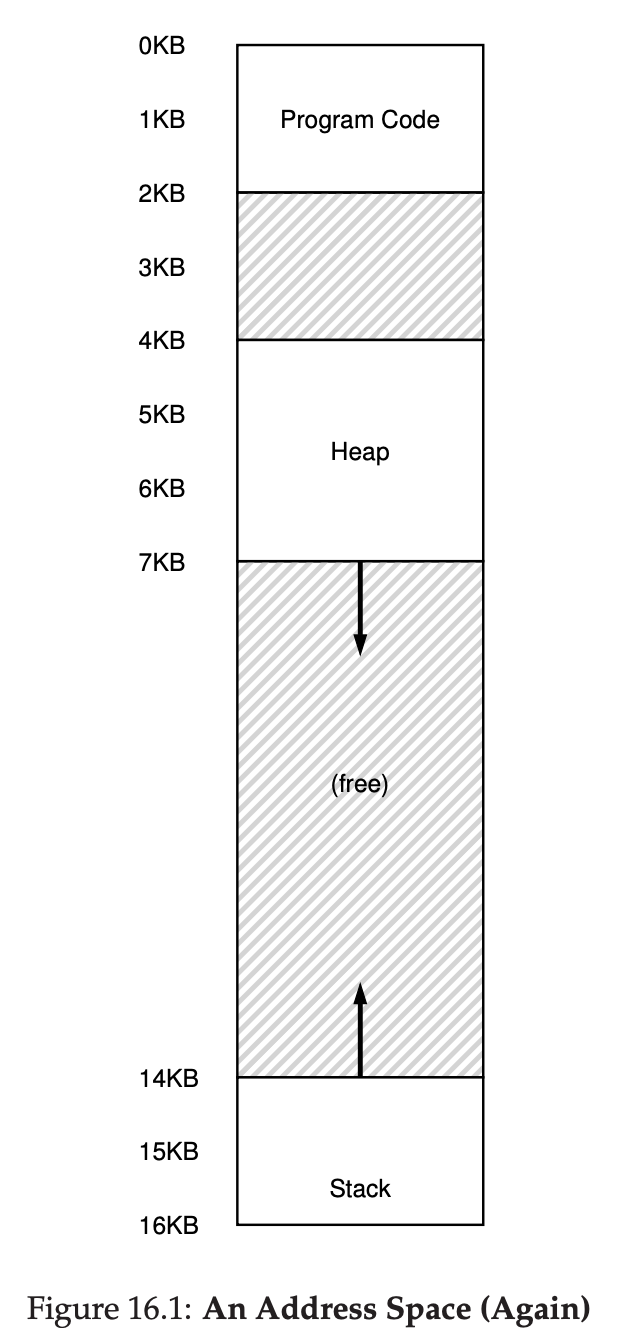
13.3 The Address Space
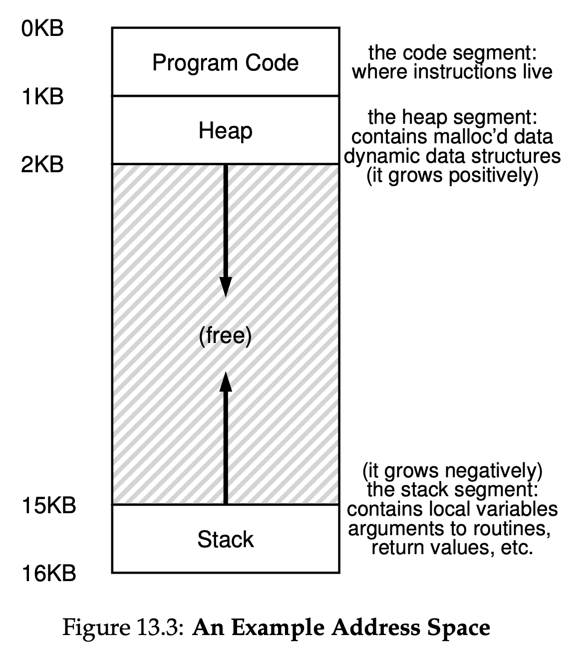
The address space of a process contains all of the memory state of the running program. For example, the code of the program(the instructions) have to live in memory somewhere, and thus they are in the address space. The program, while it is running, uses a stack to keep track of where it is in the function calll chain as well as to allocate local variables and pass parameters and return values to and from routines. Finally, the heap is used for dynamically-allocated, user-managed memory, such as that you might receive from a call to malloc() in C or new in an object-oriented language such as C++ or Java. The program code lives at the top of the address space. Code is static, so we can place it at the top of the address space and know that it won’t need any more space as the program runs. Next, we have the two regions of the address space that may grow(and shrink) while the program runs. Those are the heap(at the top) and the stack(at the bottom). We place them like this because each wishes to be able to grow, and by putting them at opposite ends of the address space, we can allow such growth: they just have to grow in opposite directions. The heap thus starts just after the code(at 1KB) and grows downward(say when a user requests more memory via malloc()); the stack starts at 16KB and grows upward(say when a user makes a procedure call).
13.4 Goals
One major goal of a virtual memory(VM) system is transparency. The OS should implement virtual memory in a way that is invisible to the running program. Thus, the program shouldn’t be aware of the fact that memory is virtualized; rahter, the program behaves as if it has its own private physical memory. Behind the scenes, the OS(and hardware) does all the work to multiplex memory among many different jobs, and hence implements the illusion. Another goal of VM is effciency. The OS should strive to make the virtualization as effcient as possible, both in terms of time(i.e., not making programs run much more slowly) and space(i.e., not using too much memory for structures needed to support virtualization). In implementing time-efficient virtualization, the OS will have to rely on hardware support, including hardware features such as TLBs. Finally, a third VM goal is protection. The OS should make sure to protect processes from one another as well as the OS itself from processes. When one process performs a load, a store, or an instruction fetch, it should not be able to access or affect in any way the memory contents of any other process or the OS itself(that is, anything outside its address space). Protection thus enables us to deliver the property of isolation among processes; each process should be running in its own isolated cocoon, safe from the ravages of other faulty or even malicious processes.
14 Interlude: Memory API
14.1 Types of Memory
In running a C program, there are two types of memory that are allocated. The first is called stack memory, and allocations and deallocations of it are managed implicitly by the compiler for you, the programmer; for this reason it is sometimes called automatic memory.
void func()
{
  int x;// declares an integer on the stack
}
It is for long-lived memory that gets us to the second type of memory, called heap memory, where all allocations and deallocations are explicitly handled by you, the programmer.
void func()
{
  int *x = (int *) malloc(sizeof(int));
}
A couple of notes about this small code snippet. First, you might notice that both stack and heap allocation occur on this line: first the compiler knows to make room for a pointer to an integer when it sees your declaration of said pointer(int *x); subsequently, when the program calls malloc(), it requests space for an integer on the heap; the routine returns the address of such an integer(upon success, or NULL on failure), which is then stored on the stack for use by the program.
14.2 The malloc() Call
The malloc() call is quite simple: you pass it a size asking for some room on the heap, and it either succeeds and gives you back a pointer to the newly-allocated space, or fails and returns NULL.
14.4 Common Errors
- Forgetting To Allocate Memory
- Not Allocating Enough Memory
- Forgetting to Initialize Allocated Memory
- Forgetting To Free Memory
- Freeing Memory Before You Are Done With It
- Freeing Memory Repeatedly
- Calling free() Incorrectly
There are really two levels of memory management in the system. The first level of memory management is performed by the OS, which hands out memory to process when they run, and takes it back when processes exit(or otherwise die). The second level of management is within each process, the operating system will reclaim all the memory of the process(including those pages for code, stack, and, as relevant here, heap) when the program is finished running. No matter what the state of your heap in your address space, the OS takes back all of those pages when the process dies, thus ensuring that no memory is lost despite the fact that you didn’t free it.
15 Mechanism: Address Translation
15.2 An Example
You can imagine the C-language representation of this code might look like this:
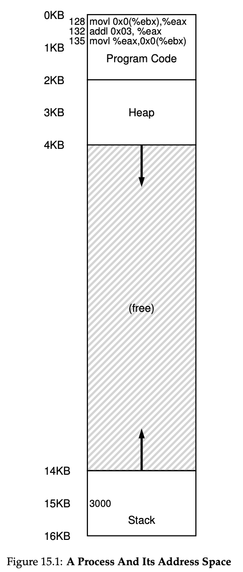
void func()
{
  int x = 3000;
  x = x + 3;
}
The compiler turns this line of code into assembly, which might look something like this(in x86 assembly).
128: movl 0x0(%ebx), %eax  ; load 0+ebx into eax
132: addl $0x03, %eax      ; add 3 to eax register
135: movl %eax, 0x0($ebx)  ; store eax back to mem
- Fetch instruction at address 128
- Execute this instruction(load from address 15 KB)
- Fetch instruction at address 132
- Execute this instruction(no memory reference)
- Fetch the instruction at address 135
- Execute this instruction(store to address 15 KB)
An example of what physical memory might look like once this process’s address space has been placed in memory is found in Figure 15.2. In this figure, you can see the OS using the first slot of physical memory for itself, and that it has relocated the process from the example above into the slot starting at physical memory address 32 KB. The other two slots are free(16 KB-32 KB and 48 KB-64 KB).
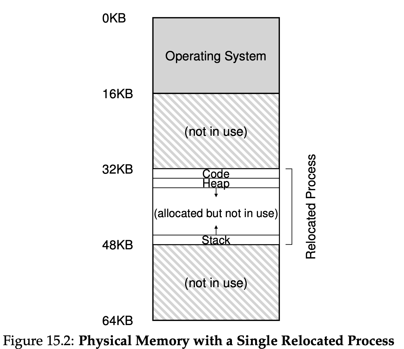
15.3 Dynamic(Hardware-based) Relocation
Specifically, we’ll need two hardware registers within each CPU: one is called the base register, and the other the bounds(sometimes called a limit register). This base-and-bounds pair is going to allow us to place the address space anywhere we’d like in physical memory, and do so while ensuring that the process can only access its own address space.
In this setup, each program is written and compiled as if it is loaded at address zero. However, when a program starts running, the OS decides where in physical memory it should be loaded and sets the base register to that value. In the example above, the OS decides to load the process at physical address 32 KB and thus sets the base register to this value. Interesting things start to happen when the process is running. Now, where any memory reference is generated by the process, it is translated by the processor in the following manner:
physical address = virtual address + baseEach memory reference generated by the process is a virtual address; the hardware in turn adds the contents of the base register to this address and the result is a physical address that can be issued to the memory system. To understand this better, let’s trace through what happens when a single instruction is executed. Specifically, let’s look at one instruction from our earlier sequence:
128: movl 0x0(%ebx), %eaxThe program counter(PC) is set to 128; when the hardware needs to fetch this instruction, it first adds the value to the base register value of 32 KB(32768) to get a physical address of 32896; the hardware then fetches the instruction from that physical address. Next, the processor begins executing the instruction. At some point, the process then issues the load from virtual address 15 KB, which the processor takes and again adds to the base register(32 KB), getting the final physical address of 47 KB and thus the desired contents. Transforming a virtual address into a physical address is exactly the technique we refer to as address translation; that is, the hardware takes a virtual address the process thinks it is referencing and transforms it into a physical address which is where the data actually resides. Because this relocation of the address happens at runtime, and because we can move address spaces even after the process has started running, the technique is often referred to as dynamic relocation.
The bounds register is there to help with protection. Specifically, the processor will first check that the memory reference is within bounds to make sure it is legal; in the simple example above, the bounds register would always be set to 16 KB. If a process generates a virtual address that is greater than the bounds, or one that is negative, the CPU will raise an exception, and the process will likely be terminated. The point of the bounds is thus to make sure that all addresses generated by the process are legal and within the “bounds” of the process.
We should note that the base and bounds registers are hardware structures kept on the chip(on pair per CPU). Sometimes people call the part of the processor that helps with address translation the memory management unit(MMU); as we develop more sophisticated memory-management techniques, we will be adding more circuitry to the MMU.
A small aside about bound registers, which can be defined in one of two ways. In one way(as above), it holds the size of the address space, and thus the hardware checks the virtual address against it first before adding the base. In the second way, it holds the physical address of the end of the address space, and thus the hardware first adds the base and then makes sure the address is within bounds. Both methods are logically equivalent; for simplicity, we’ll usually assume the former method.
15.4 hardware Support: A Summary
- The OS runs in privileged mode(or kernel mode), where it has access to the entire machine; application run in user mode, where they are limited in what they can do.
- The hardware must also provide the base and bounds registers themselves; each CPU thus has an additional pair of registers, part of the memory management unit(MMU) of the CPU.
- The hardware should provide special instructions to modify the base and bounds registers, allowing the OS to change them when different processes run. These instructions are privileged; only in kernel(or privileged)mode can the registers be modified.
- The CPU must be able to generate exceptions in situations where a user program tries to access memory illegally(with an address that is “out of bounds”); in this case, the CPU should stop executing the user program and arrange for the OS “out-of-bounds” exception handler to run.
16 Segmentation
Although the space between the stack and heap is not being used by the process, it is still taking up physical memory when we relocate the entire address space somewhere in physical memory when we relocate the entire address space somewhere in physical memory; thus, the simple approach of using a base and bounds register pair to virtualize memory is wasteful. It also makes it quite hard to run a program when the entire address space doesn’t fit into memory; thus, base and bounds is not as flexible as we would like.
16.1 Segmentaion: Generalized Base/Bounds
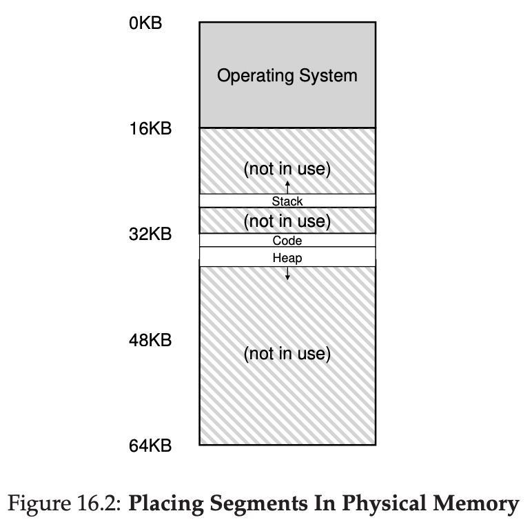
Instead of having just one base and bounds pair in our MMU, why not have a base and bounds pair per logical segment of the address space? A segment is just a contiguous portion of the address space of a particular length, and in our canonical address space, we have three logically-different segments: code, stack and heap. What segmentation allows the OS to do is to place each one of those segments in different parts of physical memory, and thus avoid filling physical memory with unsed virtual address space.
As you can see in the diagram, only used memory is allocated space in physical memory, and thus large address spaces with large amount of unused address space can be accommodated.
The term segmentation fault or violation arises from a memory access on a segmented machine to an illegal address.
16.2 Which Segment Are We Referring To?
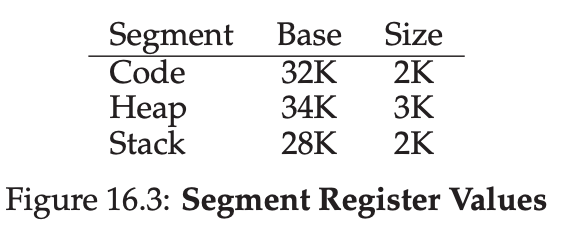
Let’s take our example heap virtual address from above(4200) and translate it, just to make sure this is clear. The virtual address 4200, in binary form, can be seen here:
As you can see from the picture, the top two bits(01) tell the hardware which segment we are referring to. The bottom 12 bits are the offset into the segment:0000 0110 1000, or hex 0x068, or 104 in decimal. Thus, the hardware simply takes the first two bits to determine which segment register to use, and then takes the next 12 bits as the offset into the segment.
You may also have noticed that when we use the top two bits, and we only have three segments(code, heap, stack), one segment of the address space goes unused. To fully utilize the virtual address space(and avoid an unused segment), some systems put code in the same segment as the heap and thus use only one bit to select which segment to use.
16.3 What About The Stack?
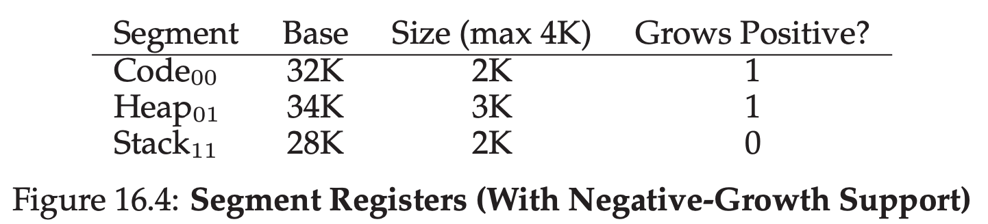
The first thing we need is a little extra hardware support. Instead of just base and bounds values, the hardware also needs to know which way the segment grows(a bit, for example, that is set to 1 when the segment grows in the positive direction, and 0 for negative). Our updated view of what the hardware tracks is seen Figure 16.4:
16.4 Support for Sharing
To support sharing, we need a little extra support from the hardware, in the form of protection bits. Basic support adds a few bits per segment, indicating whether or not a program can read or write a segment, or perhaps execute code that lies within the segment. By setting a code segment to read-only, the same code can be shared across multiple processes, without worry of harming isolation; while each process still thinks that it is accessing its own private memory, the OS is secretly sharing memory which cannot be modified by the process, and thus the illusion is preserved.
With protection bits, the hardware algorithm described earlier would also have to change. In addition to checking whether a virtual address is within bounds, the hardware also has to check whether a particular access is permissible. If a user process tries to write to a read-only segment, or execute from a non-executable segment, the hardware should raise an execption, and thus let the OS deal with the offending process.
16.6 OS Support
A program may call malloc() to allocate an object. In some cases, the existing heap will be able to service the request, and thus malloc() will find free space for the object and return a pointer to it to the caller. In others, however, the heap segment itself may need to grow. In this case, the memory-allocation library will perform a system call to grow the heap. The OS will then provide more space, updating the segment size register to the new size, and informing the library of success; the library can then allocate space for the new object and return successfully to the calling program. Do note that the OS could reject the request, if no more physical memory is available, or if it decides that the calling process already has too much.
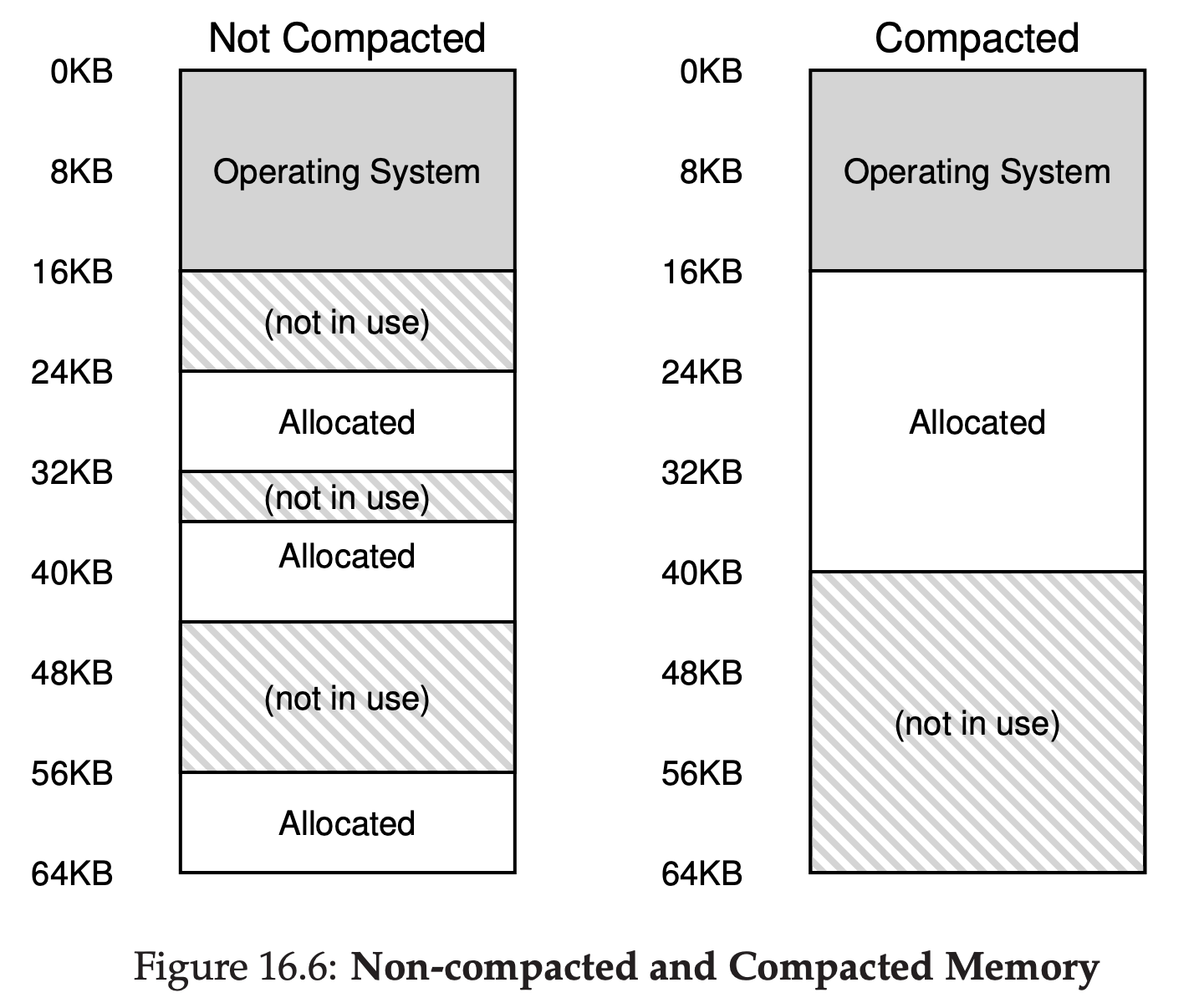
Unfortunately, though, no matter how smart the algorithm, external fragmentation(see Figure 16.6 (left)) will still exist; thus, a good algorithm simply attempts to minimize it.
17 Free-Space Management
17.1 Assumptions
void *malloc(size_t size) takes a single parameter, size, which is the number of bytes requested by the application; it hands back a pointer to a region of that size. The complementary routine void free(void *ptr) takes a pointer and frees the corresponding chunk. Note the implication of the interface: the user, when freeing the space, does not inform the library of its size; thus, the library must be able to figure out how big a chunk of memory is when handed just a pointer to it.
Allocators could also have the problem of internal fragmentation; if an allocator hands out chunks of memory bigger than that requested, any unasked for space in such a chunk is considered internal fragmentaion(because the waste occurs inside the allocated unit) and is another example of space waste.
17.2 Low-level Mechanisms
Splitting and Coalescing
A free list contains a set of elements that describe the free space still remaining in the heap. Thus, assume the following 30-byte heap:
The free list for this heap would have two elements on it. One entry describes the first 10-byte free segment(bytes 0-9), and one entry describes the other free segment(bytes 20-29):
As described above, a request for anything greater than 10 bytes will fail(returning NULL); there just isn’t a single contiguous chunk of memory of that size available. A request for exactly that size(10 bytes) could be satisfied easily by either of the free chunks. Assume we have a request for just a single byte of memory. In this case, the allocator will perform an action known as splitting: it will find a free chunk of memory that can satisfy the request and split it into two. The first chunk it will return to the caller; the second chunk will remain on the list. Thus, in our example above, if a request for 1 byte were made, and the allocator decided to use the second of the two elements on the list to satisfy the request, the call to malloc() would return 20(the address of the 1-byte allocated region) and the list would end up looking like this:
In the picture, you can see the list basically stays intact; the only change is that the free region now starts at 21 instead of 20, and the length of that free region is now just 9. Thus, the split is commonly used in allocators when requests are smaller than the size of any particular free chunk. A corollary mechanism found in many allocators is known as coalescing of free space. Take our example from above once more(free 10 bytes, used 10 bytes, and another free 10 bytes). Given this(tiny) heap, what happens when an application calls free(10), thus returning the space in the middle of the heap? If we simply add this free space back into our list without too much thinking, we might end up with a list that looks like this:
Note the problem: while the entire heap is now free, it is seemingly divided into three chunks of 10 bytes each. Thus, if a user requests 20 bytes, a simple list traversal will not find such a free chunk, and return failure. What allocators do in order to avoid this problem is coalesce free space when a chunk of memory is freed. The idea is simple: when returning a free chunk in memory, look carefully at the addresses of the chunk you are returning as well as the nearby chunks of free space; if the newly-freed space sits right next to one(or two, as in this example) existing free chunks, merge them into a single larger free chunk. Thus, with coalescing, our final list should look like this:
Indeed, this is what the heap list looked like at first, before any allocations were made. With coalescing, an allocator can better ensure that large free extents are available for the application.
Tracking The Size Of Allocated Regions
You might have noticed that the interface to free(void *ptr) does not take a size parameter; thus it is assumed that given a pointer, the malloc library can quickly determine the size of the region of memory being freed and thus incorporate the space back into the free list. To accomplish this task, most allocators store a little bit of extra information in a header block which is kept in memory, usually just before the headed-out chunk of memory. Let’s look at an example again(Figure 17.1). In this example, we are examining an allocated block of size 20 bytes, pointed to by ptr; imagine the user called malloc() and stored the results in ptr, e.g., ptr = malloc(20);. The header minimally contains the size of the allocated region(in this case, 20); it may also contain additional pointers to speed up deallocation, a magic number to provide additional integirty checking, and other information. Let’s assume a simple header which contains the size of the region and a magic number, like this:
typedef struct{
  int size;
  int magic;
} header_t;
The example above would look like what you see in Figure 17.2. When the user calls free(ptr), the library then uses simple pointer arithmetic to figure out where the header begins:
void free(void *ptr){
  header_t *hptr = (header_t *) ptr - 1;
  ...
After obtaining such a pointer to the header, the library can easily determine whether the magic number matches the expected value as a sanity check and calculate the total size of the newly-freed region via simple math(i.e., adding the size of the header to size of the region). Note the small but critical detail in the last sentence: the size of the free region is the size of the header plus the size of the space allocated to the user. Thus, when a user requests N bytes of memory, the library doesn’t search for a free chunk of size N; rather, it searches for a free chunk of size N plus the size of the header.

Embedding A Free List
Assume we have a 4096-byte chunk of memory to manage(i.e., the heap is 4KB). To manage this as a free list, we first have to initialize said list; initially, the list should have one entry, of size 4096(minus the header size). Here is the description of a node of the list:
typedef struct __node_t{
    int size;
    struct __node_t *next;
} node_t;
Now let’s look at some code that initializes the heap and puts the first element of the free list inside that space. We are assuming that the heap is built within some free space acquired via a call to the system call mmap(); this is not the only way to build such a heap but serves us well in this example. Here is the code:
// mmap() returns a pointer to a chunk of free space
node_t *head = mmap(NULL, 4096, PROT_READ|PROT_WRITE,MAP_ANON|MAP_PRIVATE, -1, 0);
head->size = 4096 - sizeof(node_t);
head->next = NULL;
After running this code, the status of the list is that it has a single entry, of size 4088. The head pointer contains the beginning address of this range; let’s assume it is 16KB. Visually, the heap thus looks like what you see in Figure 17.3.
Now, let’s imagine that a chunk of memory is requested, say of size 100 bytes. To service this request, the library will first find a chunk that is large enough to accommodate the request; because there is only one free chunk(size: 4088), this chunk will be chosen. Then, the chunk will be split into two: one chunk big enough to service the request(and header, as decribed above), and the remaining free chunk. Assuming an 8-byte header(an integer size and an integer magic number), the space in the heap now looks like what you see in Figure 17.4
Thus, upon the request for 100 bytes, the library allocated 108 bytes out of the existing one free chunk, returns a pointer(marked ptr in the figure above) to it, stashes the header information immediately before the allocated space for later use upon free(), and shrinks the one free node in the list to 3980 bytes(4088 minus 108). Now let’s look at the heap when there are three allocated regions, each of 100 bytes(or 108 including the header). A visualization of this heap is shown in Figure 17.5.
As you can see therein, the first 324 bytes of the heap are now allocated, and thus we see three headers in that space as well as three 100-byte regions being used by the calling program. The free list remains uninteresting: just a single node(pointed to by head), but now only 3764 bytes in size after the three splits. But what happens when the calling program returns some memory via free()? In this example, the application returns the middle chunk of allocated memory, by calling free(16500) (the value 16500(= 16384 + 108 + 8) is arrived upon by adding the start of the memory region, 16384(16KB = 16384Bytes), to the 108 of the previous chunk and the 8 bytes of the header for this chunk). This value is shown in the previous diagram by the pointer sptr. The library immediately figures out the size of the free region, and then adds the free chunk back onto the free list. Assuming we insert at the head of the free list, the space now looks like this(Figure 17.6).
Now we have a list that starts with a small free chunk(100 bytes, pointed to by the head of the list) and a large free chunk(3764 bytes). Our list finally has more than one element on it! And yes, the free space is fragmented, an unfortunate but common occurrence. One last example: let’s assume now that the last two in-use chunks are freed. Without coalescing, you end up with fragmentation(Figure 17.7).
As you can see from the figure, we now have a big mess! Why? Simple, we forgot to coalesce the list. Although all of the memory is free, it is chopped up into pieces, thus appearing as a fragmented memory despite not being one. The solution is simple: go through the list and merge neighboring chunks; when finished, the heap will be whole again.
17.3 Basic Strategies
Best Fit
Search through the free list and find chunks of free memory that are as big or bigger than the requested size. Then, return the one that is the smallest in that group of candidates. However, there is a cost; naive implementations pay a heavy performance penalty when performing an exhaustive search for the correct free block.
Worst Fit
Find the largest chunk and return the requested amount; keep the remaining(large) chunk on the free list. Worst fit tries to thus leave big chunks free instead of lots of small chunks that can arise from a best-fit approach. However, a full search of free space is required, and thus this approach can be costly.
First Fit
Find the first block that is big enough and returns the requested amount to the user. First fit has the advantage of speed - no exhaustive search of all the free spaces are necessary - but sometimes pollutes the beginning of the free list with small objects.
Next Fit
Keep an extra pointer to the location within the list where one was looking last. The idea is to spread the searches for free space throughout the list more uniformly,thus avoiding splintering of the beginning of the list. An exhaustive search is once again avoided.
18 Pagine: Introduction
Instead of splitting up a process’s address space into some number of variable-size logical segments(e.g., code,heap,stack), we divide it into fixed-sized units, each of which we call a page. Correspondingly, we view physical memory as an array of fixed-sized slots called page frame; each of these frames can contain a single virtual-memory page.
18.1 A simple Example And Overview
Figure 18.1 presents an example of a tiny address space, only 64 bytes total in size, with four 16-byte pages(virtual pages 0,1,2,3).
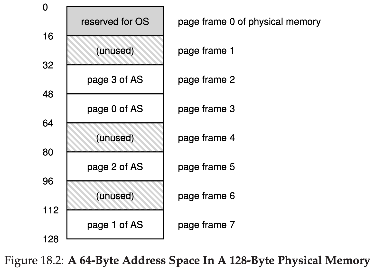
Physical memory, as shown in Figure 18.2, also consists of a number of fixed-sized slot, in this case eight page frames. As you can see in the diagram, the pages of the virtual address space have been placed at different locations throughout physical memory; the diagram also shows the OS using some of physical memory for itself.
The most important improvement of paging will be flexibility: with a fully-developed paging approach, the system will be able to support the abstraction of an address space effectively, regardless of how a process uses the address space; we won’t make assumptions about the direction the heap and stack grow and how they are used. Another advantage is the simplicity of free-space management that paging affords. When the OS wishes to place our tiny 64-byte address space into our eight-page physical memory, it simply finds four free pages; perhaps the OS keeps a free list of all free pages for this, and just grabs the first four free pages off of this list.
To record where each virtual page of the address space is placed in physical memory, the operating system usually keeps a per-process data structure known as a page table. The major role of the page table is to store address translations for each of the virtual pages of the address space, thus letting us know where in physical memory each page resides.
It is important to remember that this page table is a per-process data structure. If another process were to run in our example above, the OS would have to manage a different page table for it, as its virtual pages obviously map to different physical pages.
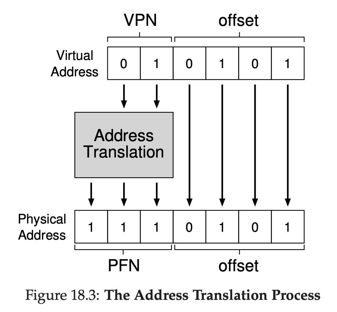
mvol <virtual address>, %eaxTo translate this virtual address that the process generated, we have to first split it into two components: the virtual page number(VPN), and the offset within the page. For this example, because the virtual address space of the process is 64 bytes, we need 6 bits total for our virtual address($2^{6}$ = 64). Thus, our virtual address can be conceptualized as follows:
In this diagram, Va5 is the highest-order bit of the virtual address, and Va0 the lowest-order bit. Because we know the page size(16 bytes), we can further divide the virtual address as follows:
The page size is 16 bytes in a 64-byte address space; thus we need to be able to select 4 pages, and the top 2 bits of the address do just that. Thus, we have a 2-bit virtual page number(VPN). The remaining bits tell us which byte of the page we are interested in, 4 bits in this case; we call this the offset. When a process generates a virtual address, the OS and hardware must combine to translate it into a meaningful physical address.
18.2 Where Are Page Tables Stored?
Because page tables are so big, we don’t keep any special on-chip hardware in the MMU to store the page table of the currently-running process. Instead, we store the page table for each process in memory somewhere.
19 Paging: Faster Translations(TLBs)
Upon each virtual memory reference, the hardware first checks the TLB(translation-lookaside buffer) to see if the desired translation is held therein; if so, the translation is performed(quickly) without having to consult the page table(which has all translations).
19.1 TLB Basic Algorithm
The TLB, like all cache, is built on the premise that in the common case, translations are found in the cache. If so, little overhead is added, as the TLB is found near the processing core and is designed to be quite fast. When a miss occurs, the high cost of paging is incurred; the page table must be accessed to find the translation, and an extra memory reference result. If this happen often, the program will likely run noticeably more slowly; memory accesses, relative to most CPU instructions, are quite costly, and TLB misses lead to more memory accesses. Thus, it is our hope to avoid TLB misses as much as we can.
19.3 Who Handles The TLB Miss?
In the olden days, the hardware had complex instruction sets and would handle the TLB miss entirely. More modern architectures have what is known as a software-managed TLB. On a TLB miss, the hardware simply raise an exception, which pauses the current instruction stream, raise the privilege level to kernel mode, and jumps to a trap handler.
The primary advantage of the software-managed approach is flexiblity: the OS can use any data structure it wants to implement the page table, without necessitating hardware change. Another advantage is simplicity, the hardware doesn’t do much on a miss: just raise an exception and let the OS TLB miss handler do the rest.
19.4 TLB Contents: What’s In There?
A typical TLB might have 32, 64, or 128 entries and be what is called fully associative. Basically, this just means that any given translation can be anywhere in the TLB, and that the hardware will search the entire TLB in parallel to find the desired translation. A TLB entry might look like this:
VPN | PFN | other bits
19.5 TLB Issue: Context Switches
The TLB contains virtual-to-physical translations that are only valid for the currently running process. As a result, when switching from one process to another, the hardware or OS(or both) must be careful to ensure that the about-to-be-run process does not accidentally use translations from some previously run process.
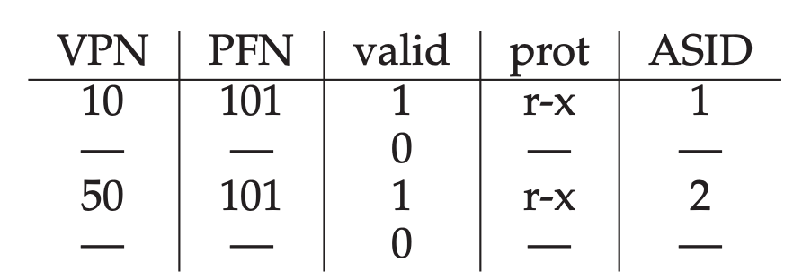
Some systems add hardware support to enable sharing of the TLB across context switches. In particular, some hardware systems provide an address space identifier(ASID) field in the TLB. You can think of the ASID as a process identifier(PID), but usually it has fewer bits.
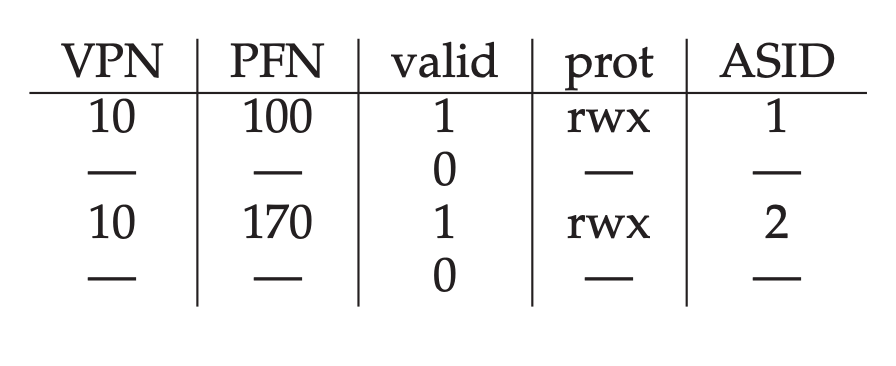
When two processes share a page(a code page). In the example above, Process 1 is sharing physical page 101 with process 2; P1 maps this page into the 10th page of its address space, whereas P2 maps it to the 50th page of its address space. Sharing of code pages(in binary, or shared libraries) is useful as it reduces the number of physical pages in use, thus reducing memory overheads.
20 Paging: Smaller Tables
20.1 Simple Solution: Bigger Pages
We could reduce the size of the page table in one simple way: use bigger pages. The major problem with this approach, however, is that big pages lead to waste within each page, a problem known as internal fragmentaion. Applications thus end up allocating pages but only using little bits and pieces of each, and memory quickly fills up with these overly-large pages.
20.2 Hybrid Approach: Paging and Segments
Instead of having a single page table for the entire address space of the process, why not have one per logical segment?
Remember with segmentation, we had a base register that told us where each segment lived in physical memory, and a bound or limit register that told us the size of said segment. In our hybrid, we still have those structures in the MMU; here, we use the base not to point to the segment itself but rather to hold the physical address of the page table of that segment. The bounds register is used to indicate the end of the page table(i.e., how many valid pages it has). Let’s do a simple example of clarify. Assume a 32-bit virtual address space with 4KB pages, and an address space split into four segments. We’ll only use three segments for this example: one for code, one for heap, one for stack. To determine which segment an address refers to, we’ll use the top two bits of the address space. Let’s assume 00 is the unused segment, with 01 for code, 10 for the heap, and 11 for the stack. Thus, a virtual address looks like this:
In the hardware, assume that there are thus three base/bounds pairs, one each for code,heap, and stack. When a process is running, the base register for each of these segments contains the pyhsical address of a linear page table for the segment; thus, each process in the system now has three page tables associated with it. On a context switch, there registers must be changed to reflect the location of the page tables of the newly-running process.
The critical difference in our hybrid scheme is the presence of a bounds register per segment; each bounds register holds the value of the maximum valid page in the segment. For example, if the code segment is using its first three pages(0,1 and 2), the code segment page table will only have three entries allocated to it and the bounds register will be set to 3; memory accesses beyond the end of the segment will generate an exception and likely lead to the termination of the process.
20.3 Multi-level Page Tables
The basic idea behind a multi-level page table is simple. First, chop up the page table into page-sized unit; then, if an entire page of page-table entries(PTFs) is invalid, don’t allocate that page of the page table at all. To track whether a page of the page table is valid(and if valid, where it is in memory), use a new structure, called the page directory. The page directory thus either can be used to tell you where a page of the page table is, or that the entire page of the page table contains on valid pages.
Figure 20.3 shows an example. On the left of the figure is the classic linear page table; even though most of the middle regions of the address space are not valid, we still require page-table space allocated for those regions(i.e., the middle two pages of the page table). On the right is a multi-level page table. The page directory marks just two pages of the page table as valid(the first and last); thus, just those two pages of the page table reside in memory. And thus you can see one way to visualize what a multi-level table is doing: it just makes parts of the linear page table disappear(freeing those frames for other uses), and tracks which pages of the page table are allocated with the page directory.
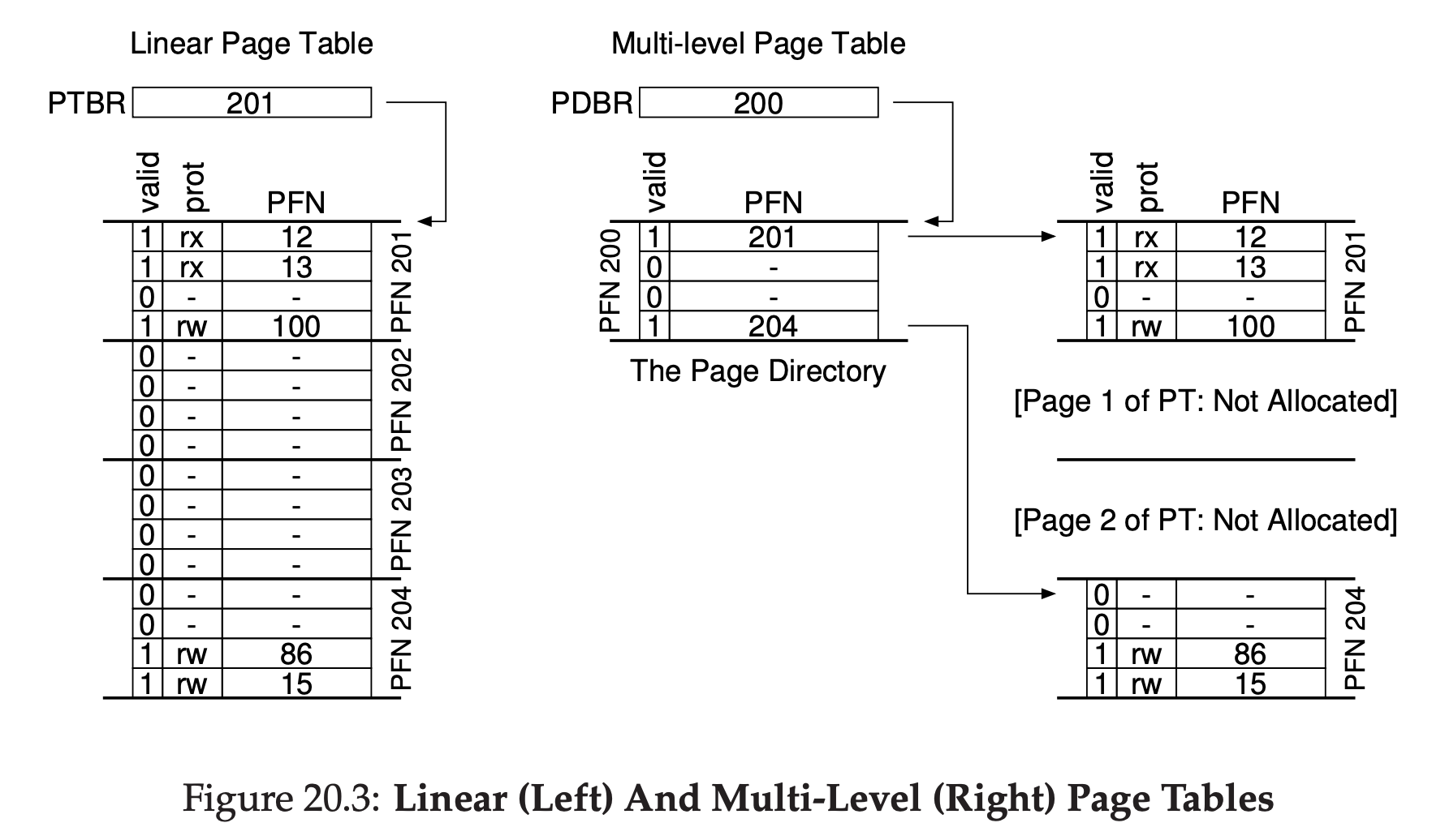
The page directory, in a simple two-level table, contains one entry per page of the page table. It consists of a number of page directory entries(PDE). A PDE has a valid bit and a page frame number, similar to a PTE.
Multi-level page tables have some obvious advantages over approaches we’ve seen thus far. First, and perhaps most obviously, the multi-level table only allocates page-table space in proportion to the amount of address space you are using; thus it is generally compact and support sparse address spaces. Second, if carefully constructed, each portion of the page table fits neatly within a page, making it easier to manage memory; the OS can simply grab the next free page when it needs to allocate or grow a page table. Contrast this to a simple linear page table, which is just an array of PTEs indexed by VPN; with such a structure, the entire linear page table must reside contiguously in physical memory.
It should be noted that there is a cost to multi-level tables; on a TLB miss, two loads from memory will be required to get the right translation information from the page table( one for the page directory, and one for the PTE itself), in constrast to just one load with a linear page table. Thus, the multi-level table is a small example of a time-space trade-off. We wanted smaller tables(and got them), but not for free; although in the common case(TLB hit), performance is obviously identical, a TLB miss suffers from a higher cost with this smaller table. Another obvious negative is complexity. Whether it is the hardware or OS handling the page-table lookup(on a TLB miss), doing so is undoubtedly more involved than a simple linear page-table lookup. Often we are willing to increase complexity in order to improve performance or reduce overheads; in the case of a multi-level table, we make page-table lookups more complicated in order to save valuable memory.
21 Beyond Physical Memory: Mechanisms
21.1 Swap Space
The first thing we will need to do is to reserve some space on the disk for moving pages back and forth. In operating systems, we generally refer to such space as swap space, because we swap pages out of memory to it and swap pages into memory from it.
21.2 The Present Bit
When the hardware looks in the PTE, it may find that the page is not present in physical memory. The way the hardware determines this is through a new piece of information in each page-table entry, known as the present bit. If the present bit is set to one, it means the page is present in physical memory and everything proceeds as above; if it is set to zero, the page is not in memory but rather on disk somewhere. The act of accessing a page that is not in physical memory is commonly referred to as a page fault.
21.3 The Page Fault
Recall that with TLB misses, we have two types of systems: hardware-managed TLBs and software-managed TLBs. In either type of system, if a page is not present, the OS is put in charge to handle the page fault. The appropriately-named OS page-fault handler runs to determine what to do. Virtually all systems handle page faults in software; even with a hardware-managed TLB, the hardware trusts the OS to manage this important duty.
When the OS receives a page fault for a page, it looks in the PTE to find the address, and issue the request to disk to fetch the page into memory. When the disk I/O completes, the OS will then update the page table to mark the page as present, update the PFN field of the page-table entry to record the in-memory location of the newly-fetched page, and retry the instruction. This next attempt may generate a TLB miss, which would then be serviced and update the TLB with the translation. Finally, a last restart would find the translation in the TLB and thus proceed to fetch the desired data or instruction from memory at the translated physical address.
Note that while the I/O is flight, the process will be in the blocked state. Thus, the OS will be free to run other ready processes while the page fault is being serviced. Because I/O is expensive, this overlap of the I/O(page fault) of one process and the execution of another is yet another way a mulitprogrammed system can make the most effective use of its hardware.
21.5 Page Fault Control Flow
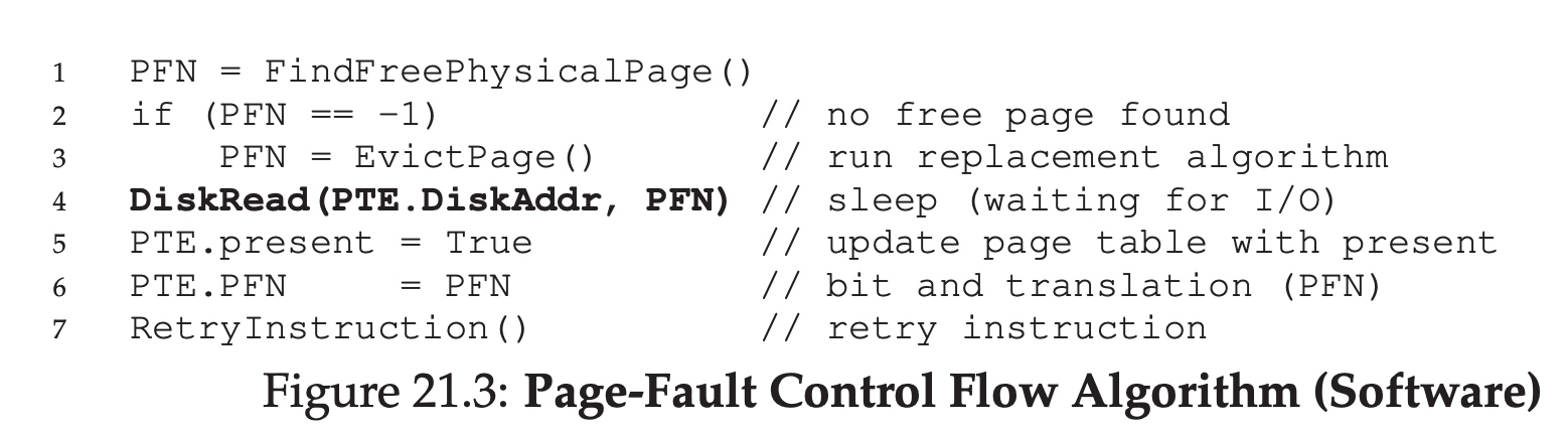
From the sofeware control flow in Figure 21.3, we can see what the OS roughly must do in order to service the page fault. First, the OS must find a physical frame for the soon-to-be-faulted-in page to reside within; if there is no such page, we’ll have to wait for the replacement algorithm to run and kick some pages out of memory, thus freeing them for use here. With a physical frame in hand, the handler then issues the I/O request to read in the page from swap space. Finally, when that slow operation completes, the OS updates the page table and retries the instruction. The retry will result in a TLB miss, and then, upon another retry, a TLB hit, at which point the hardware will be able to access the desired item.
21.6 When Replacements Really Occur
There are many reasons for the OS to keep a small portion of memory free more proactively. To keep a small amount of memory free, most operating systems thus have some kind of high watermark(HW) and low watermark(LW) to help decide when to start evicting pages from memory. How this works is as follows: when the OS notices that there are fewer than LW pages available, a background thread that is responsible for freeing memory runs. The thread evicts pages until there are HW pages available. The background thread, sometimes called the swap daemon or page daemon, then goes to sleep, happy that it has freed some memory for running processes and the OS to use.
22 Beyond Physical Memory: Policies
Knowing the number of cache hits and misses let us calculate the average memory access time(AMAT) for a program. Specifically, given these values, we can compute the AMAT of a program as follows: AMAT = $T_{M}$ + ($P_{Miss}$ · $T_{D}$) where $T_{M}$ represents the cost of accessing memory, $T_{D}$ the cost of accessing disk, and $P_{Miss}$ the probability of not finding the data in the cache(a miss); $P_{Miss}$ varies from 0.0 to 1.0, and sometimes we refer to a percent miss rate instead of a probability. Note you always pay the cost of accessing the data in memory; when you miss, however, you must additionally pay the cost of fetching the data from disk.
22.2 The Optimal Replacement Policy
The optimal replacement policy leads to the fewest number of misses overall. Replacing the page that will be accessed furthest in the future is the optimal policy, resulting in the fewest-possible cache misses.
If you have to throw out some page, why not throw out the one that is needed the furthest from now? By doing so, you are essentially saying that all the other pages in the cache are more important than the one furthest out. The reason this is true is simple: you will refer to the other pages before you refer to the one furthest out.
Unfortunately, as we saw before in the development of scheduling policies, the future is not generally known; you can’t build the optimal policy for a general-purpose operating system. Thus, in developing a real, deployable policy, we will focus on approaches that find some other way to decide which page to evict. The optimal policy will thus serve only as a comparision point, to know how close we are to “perfect”.
22.3 A Simple Policy: FIFO
Some system used FIFO replacement, where pages were simply placed in a queue when they enter the system; when a replacement occurs, the page on the tail of the queue(the “first-in” page) is evicted. FIFO has one great strength: it is quite simple to implement.
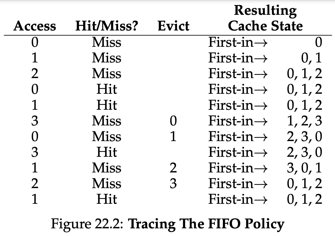
Comparing FIFO to optimal, FIFO does notably worse: a 36.4% hit rate(or 57.1% excluding compulsory misses). FIFO simply can’t determine the importance of blocks: even though page 0 had been accessed a number of times, FIFO still kicks it out, simply because it was the first one brought into memory.
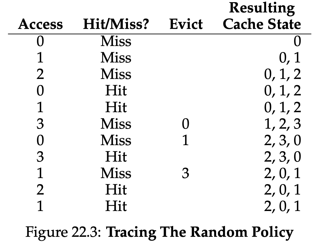
22.4 Another Simple Policy: Random
Random policy simply picks a random page to replace under memory pressure. Random has properties similar to FIFO; it is simple to implement, but it doesn’t really try to be too intelligent in picking which blocks to evict. Of course, how Random does depends entirely upon how lucky(or unlucky) Random gets in its choices.
22.5 Using History: LRU
Unfortunately, any policy as simple as FIFO or Random is likely to have a common problem: it might kick out an important page, one that is about to be referenced again.
As we did with scheduling policy, to improve our guess at the future, we once again lean on the past and use history as our guide.
One type of historical information a page-replacement policy could use is frequency; if a page has been accessed many times, perhaps it should not be replaced as it clearly has some value. A more commonly-used property of a page is its recency of access; the more recently a page has been accessed, perhaps the more likely it will be accessed again.
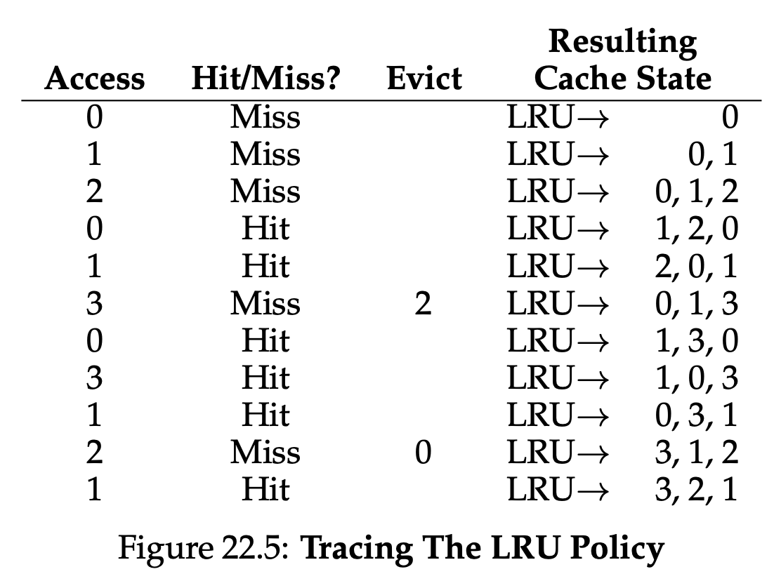
This family of policies is based on what people refer to as the principle of locality, which basically is just an observation about programs and their behavior. What this principle says, quite simply, is that programs tend to access certain code sequences(e.g., in a loop) and data structures(e.g., an array accessed by the loop) quite frequently; we should thus try to use history to figure out which pages are important, and keep those pages in memory when it comes to eviction time. And thus, a family of simple historically-based algorithms are born. The Least-Frequently-Used(LFU) policy replaces the least-frequently-used page when an eviction must take place. Similarly, the Least-Recently-Used(LRU) policy replaces the least-recently-used page.
From the figure, you can see how LRU can use history to do better than stateless polices such as Random or FIFO. Thus, LRU does as well as possible , matching optimal in its performance.
22.6 Workload Example
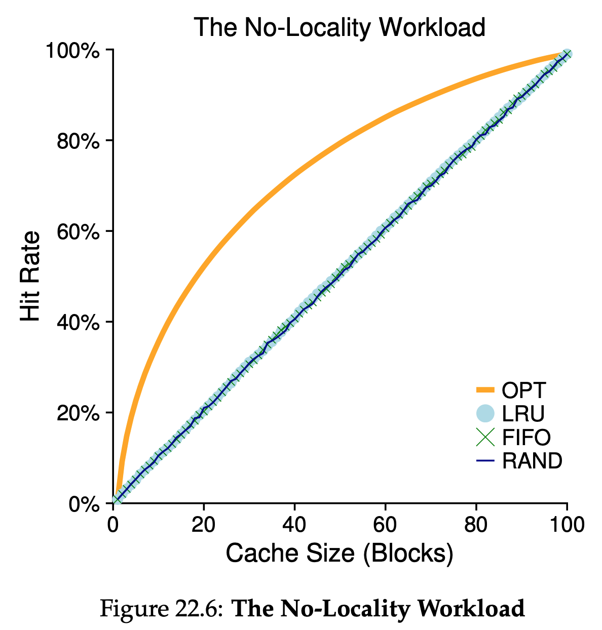
We can draw a number of conclusions from the Figure 22.6. First, when there is no locality in the workload, it doesn’t matter much which realistic policy you are using; LRU, FIFO, and Random all perform the same, with the hit rate exactly determined by the size of the cache, Second, when the cache is large enough to fit the entire workload, it also doesn’t matter which policy you use; all policies(even Random) converge to a 100% hit rate when all the referenced blocks fit in cache. Finally, you can see that optimal performs noticeably better than the realistic policies; peeking into the future, if it were possible, does a much better job of replacement.
“80-20” workload exhibits locality: 80% of the references are made to 20% of the pages(the “hot” pages); the remaining 20% of the references are made to the remaining 80% of the pages(the “cold” pages). As you can see from the figure, which both random and FIFO do reasonably well, LRU does better, as it is more likely to hold onto the hot pages; as those pages have been referred to frequently in the past, they are likely to be referred to again in the near future. Optimal once again does better, showing that LRU’s historical information is not perfect.
You might now be wondering: is LRU’s improvement over Random and FIFO really that big of a deal? The answer, as usual, is “it depends.” If each miss is very costly(not uncommon), then even a small increase in hit rate(reduction in miss rate) can make a huge difference on performance. If misses are not so costly, then of course the benifits possible with LRU are not nearly as important.
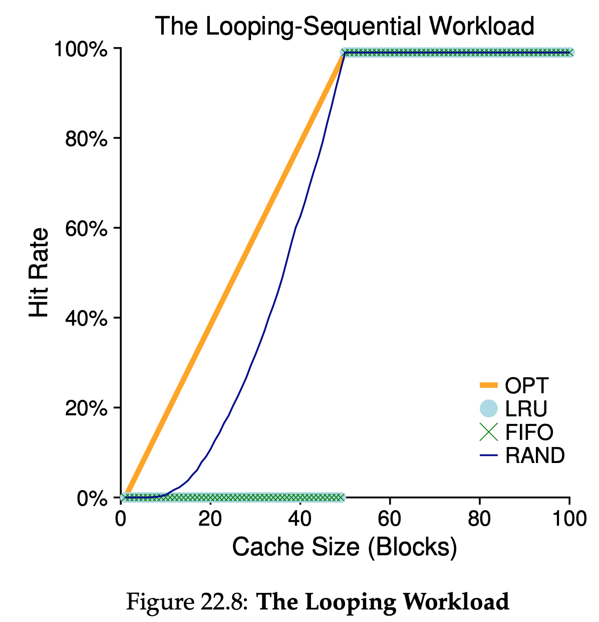
We refer to “looping sequential” workload as 50 pages in sequence, starting at 0, then 1,…, up to page 49, and then we loop, repeating those accesses, for a total of 10,000 accesses to 50 unique pages. This workload, common in many applications(including important commercial applications such as databases), represents a worst-case for both LRU and FIFO. These algorithms, under a looping-sequential workload, kick out older pages; unfortunately, due to the looping nature of the workload, these older pages are going to be accessed sooner than the pages that the policies prefer to keep in cache. Indeed, even with a cache of size 49, a looping-sequential workload of 50 pages results in a 0% hit rate. Interestingly, Random fares notably better, not quite approaching optimal, but at least achieving a non-zero hit rate. Turns out that random has some nice properties; one such property is not having weird corner-case behaviors.
22.7 Implementing Historical Algorithms
To implement LRU perfectly, we need to do a lot of work. Specifically, upon each page access, we must update some data structure to move this page to the front of the list. Contrast this to FIFO, where the FIFO list of pages is only accessed when a page is evicted or when a new page is added to the list. To keep track of which pages have been least-and most-recently used, the system has to do some accounting work on every memory reference. Clearly, without great care, such accounting could greatly reduce performance.
22.8 Approximately LRU
Approximating LRU is more feasible from a computational-overhead standpoint, and indeed it is what many modern system do. The idea requires some hardware support, in the form of a use bit(sometimes called the reference bit). There is one use bit per page of the system, and the use bits live in memory somewhere. Whenever a page is referenced(i.e., read or write), the use bit is set by hardware to 1. The hardware never clears the bit, though(i.e., sets it to 0); that is the responsibility of the OS. One simple approach, clock algorithm, was suggested. Imagine all the pages of the system arranged in a circular list. A clock hand points to some paritcular page to begin with. When a replacement must occur, the OS checks if the currently-pointed to page P has a use bit of 1 or 0. If 1, this implies that page P was recently used and thus is not a good candidate for replacement. Thus, the use bit for P is set to 0(cleared), and the clock hand is incremented to the next page(P+1). The algorithm continues until it finds a use bit that is set to 0, implying this page has not been recently used(or, in the worst case, that all pages have been and that we have now searched through the entire set of pages, clearing all the bits).
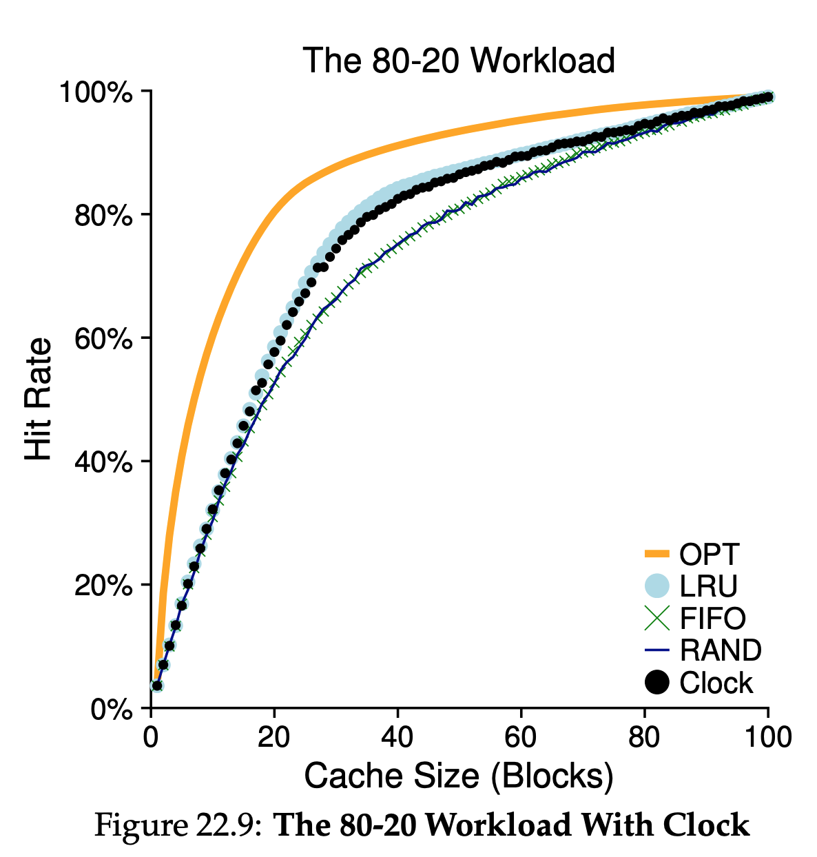
22.9 Considering Dirty Pages
One small modification to the clock algorithm that is commonly made is the additional consideration of whether a page has been modified or not while in memory. The reason for this: if a page has been modified and is thus dirty, it must be written back to disk to evict it, which is expensive. If it has not been modified(and is thus clean), the eviction is free; the physical frame can simply be reused for other purposes without additional I/O. Thus, some VM systems prefer to evict clean pages over dirty pages. To support this behavior, the hardware should include a modified bit(a.k.a dirty bit). This bit is set any time a page is written, and thus can be incorporated into the page-replacement algorithm. The clock algorithm, for example, could be changed to scan for pages that are both unused and clean to evict first; failing to find those, then for unused pages that are dirty, and so forth.
20.10 Other VM Policies
For most pages, the OS simply uses demand paging, which means the OS brings the page into memory when it is accessed, “on demand” as it were. Of course, the OS could guess that a page is about to be used, and thus bring it in ahead of time; this behavior is known as prefetching and should only be done when where is reasonable chance of success. Another policy determines how the OS writes pages out to disk. Of course, they could simply be written out one at a time; however, many systems instead collect a number of pending writes together in memory and write them to disk in one(more effcient) write. This behavior is usually called clustering or simply grouping of writes, and is effective because of the nature of disk drives, which perform a single large write more effciently than many small ones.
23 Complete Virtual Memory Systems
23.1 VAX/VMS Virtual Memory
WHY NULL POINTER ACCESSES CAUSE SEG FAULTS You shold now have a good understanding of exactly what happens on a null-pointer dereference. A process generates a virtual address of 0, by doing something like this:
int *p = NULL; //set p = 0
*p = 10;       // try to store 10 to virtual addr 0
The hardware tries to look up the VPN(also 0 here) in the TLB, and suffers a TLB miss. The page table is consulted, and the entry for VPN 0 is found to be marked invalid. Thus, we have an invalid access, which transfers control to the OS, which likely terminates the process(on UNIX system, processes are sent a signal which allows them to react to such a fault; if uncaught, however, the process is killed).
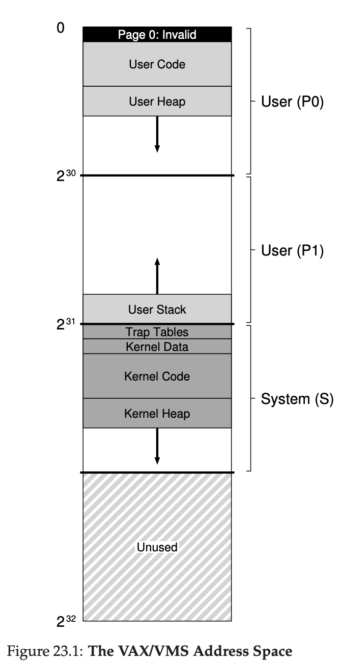
23.2 The Linux Virtual Memeory System
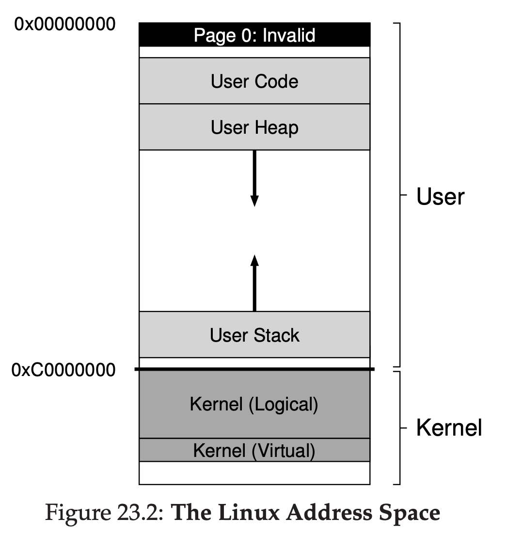
26 Concurrency: An Introduction
Instead of our classic view of a single point of execution within a program(i.e., a single PC where instructions are being fetched from and executed), a multi-threaded program has more than one point of execution(i.e., multiple PCs, each of which is being fetched and executed from). Perhaps another way to think of this is that each thread is very much like a separate process, except for one difference: they share the same address space and thus can access the same data.
The state of a single thread is thus very similar to that of a process. It has a program counter(PC) that tracks where the program is fetching instructions from. Each thread has its own private set of registers it uses for computation; thus, if there are two threads that are running on a single processor, when switching from running one(T1) to running the other(T2), a context switch must take place. The context switch between threads is quite similar to the context switch between processes, as the register state of T1 must be saved and the register state of T2 restored before running T2. With processes, we saved state to a process control block(PCB); now, we’ll need one or more thread control blocks(TCBs) to store the state of each thread of a process. There is one major difference, though, in the context switch we perform between threads as compared to processes: the address space remains the same(i.e., there is no need to switch which page table we are using). One other major difference between threads and processes concerns the stack. In our simple model of the address space of a classic process(which we can now call a single-threaded process), there is a single stack, usually residing at the bottom of the address space.(Figure 26.1, left). However, in multi-threaded process, each thread runs independently and of course may call into various routines to do whatever work it is doing. Instead of a single stack in the address space, there will be one per thread. Let’s say we have a multi-threaded process that has two threads in it; the resulting address space looks different(Figure 26.1, right). In this figure, you can see two stacks spread throughout the address space of the process. Thus, any stack-allocated variables, parameters, return values, and other things that we put on the stack will be placed in what is sometimes called thread-local storage, i.e., the stack of the relevant thread.
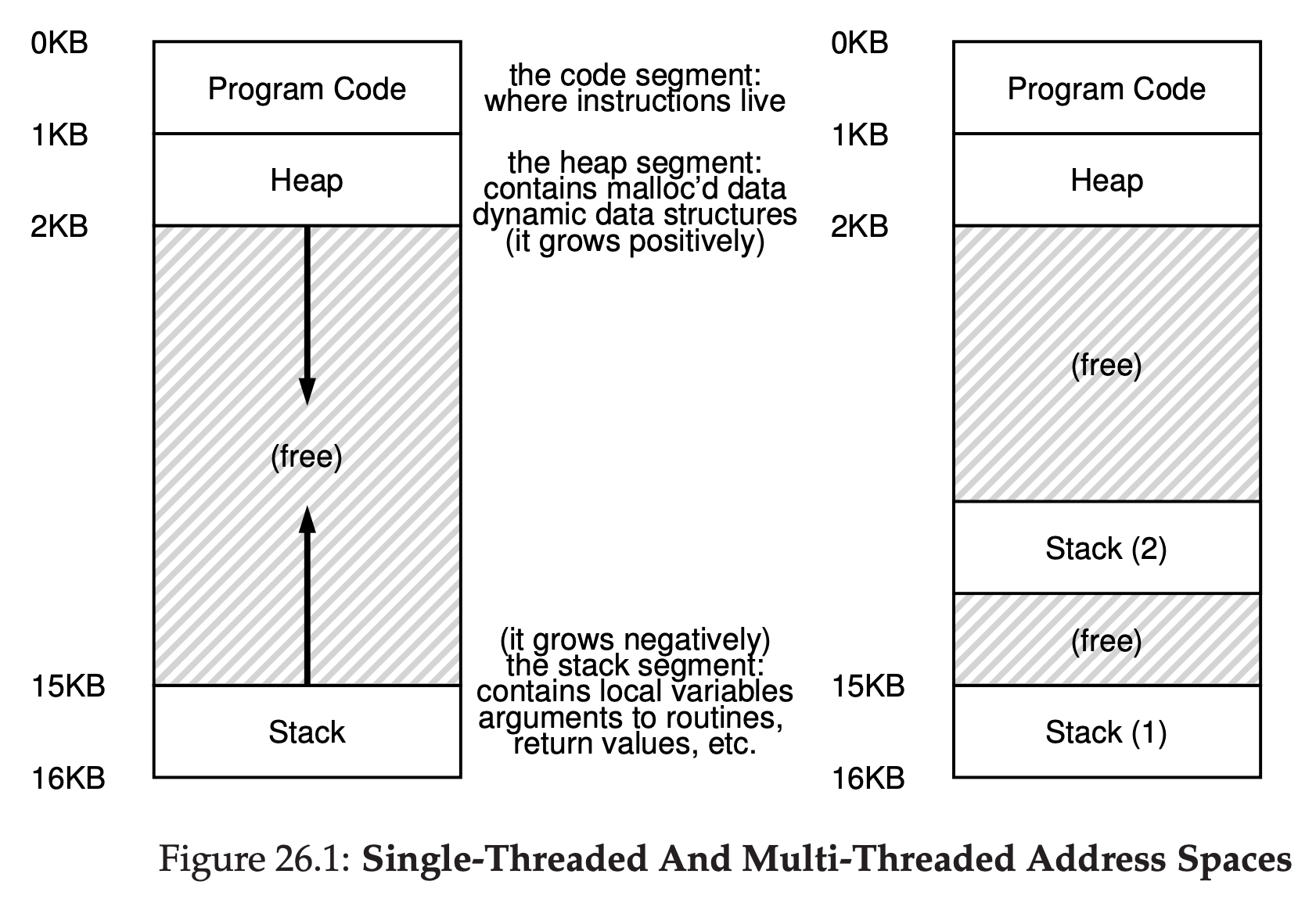
26.1 Why Use Threads?
As it turns out, there are at least two major reasons you should use threads. The first is simple: parallelism. Imagine you are writing a program that performs operations on very large arrays, for example, adding two large arrays together, or incrementing the value of each element in the array by some amount. If you are running on just a single processor, the task is straightforward: just perform each operation and be done. However, if you are executing the program on a system with mulitple processors, you have the potential of speeding up this process considerably by using the processors to each perform a portion of the work. The task of transforming your standard single-threaded program into a program that does this sort of work on multiple CPUs is called parallelization, and using a thread per CPU to do this work is a natural and typical way to make programs run faster on modern hardware. The second reason is a bit more subtle: to avoid blocking program progress due to slow I/O. Imagine that you are writing a program that performs different types of I/O: either waiting to send or receive a message, for an explicit disk I/O to complete, or even(implicitly) for a page fault to finish. Instead of waiting, your program may wish to do something else, inluding utilizing the CPU to perform computation, or even issuing further I/O requests. Using threads is a natural way to avoid getting stuck; while one thread in your program waits(i.e., is blocked waiting for I/O), the CPU sheduler can switch to other threads, which are ready to run and do something useful. Threading enables overlap of I/O with other activities within a single program, much like multiprogramming did for processes across programs; as a result, many modern server-based applications(web servers, database management systems, and the like) make use of threads in their implementations. Of course, in either of the cases mentioned above, you could use multiple processes instead of threads. However, threads share an address space and thus make it easy to share data, and hence are a natural choice when constructing these types of programs. Processes are a more sound choice for logically separate tasks where little sharing of data structures in memory is needed.
27 Interlude: Thread API
28 Locks
28.1 Locks: The Basic Idea
A lock is just a variable, and thus to use one, you must declare a lock variable of some kind(such as mutex above). This lock variable(or just “lock” for short) holds the state of the lock at any instant in time. It is either available(or unlocked or free) and thus no thread holds the lock, or acquired(or locked or held), and thus exactly one thread holds the lock and presumably is in a critical section.
The semantics of the lock() and unlock() rontines are simple. Calling the routine lock() tries to acquire the lock; if no other thread holds the lock(i.e., it is free), the thread will acquire the lock and enter the critical section; this thread is sometimes said to be the owner of the lock. If another thread then call lock() on that same lock variable(mutex in this example), it will not return while the lock is held by another thread; in this way, other threads are prevented from entering the critical section while the first thread that holds the lock is in there. Once the owner of the lock calls unlock(), the lock is now available(free) again. If no other threads are waiting for the lock(i.e., no other thread has called lock() and is stuck therein), the state of the lock is simply changed to free. If there are waiting threads(stuck in lock()), one of them will(eventually) notice(or be informed of) this change of the lock’s state, acquire the lock, and enter the critical section.
In general, we view threads as entities created by the programmer but scheduled by the OS, in any fashion that the OS chooses.
28.2 Pthread Locks
The name that the POSIX library uses for a lock is a mutex, as it is used to provide mutual exclusion between threads, i.e., if one thread is in the critical section, it excludes the others from entering until it has completed the section.
28.4 Evaluating Locks
The first is whether the lock does its basic task, which is to provide mutual exclusion. The second is fairness. Does each thread contending for the lock get a fair shot at acquiring it once it is free? Another way to look at this is by examining the more extreme case: does any thread contending for the lock starve while doing so, thus never obtaining it? The final criterion is performance, specifically the time overheads added by using the lock.
28.5 Controlling Interrupts
One of the earliest solutions used to provide mutual exclusion was to disable interrupts for critical sections; this solution was invented for single-processor systems. The code would look like this:
void lock(){
   DisableInterrupts();
}
void unlock(){
   EnableInterrupts();
}
28.6 A Failed Attempt: Just Using Loads/Stores
Using a simple variable(flag) to indicate whether some thread has possession of a lock. The first thread that enters the critical section will call lock(), which tests whether the flag is equal to 1, and then sets the flag to 1 to indicate that the thread now holds the lock. When finished with the critical section, the thread calls unlock() and clears the flag, thus indicating that the lock is no longer held. If another thread happens to call lock() while that first thread is in the critical section, it will simply spin-wait in the while loop for that thread to call unlock() and clear the flag. Once that first thread does so, the waiting thread will fall out of the while loop, set the flag to 1 for itself, and proceed into the critical section.
typedef struct __lock_t { int flag;} lock_t;

void init(lock_t *mutex) {
  // 0 -> lock is available, 1 -> held
  mutex->flag = 0;
}

void lock(lock_t *mutex) {
  while(mutex->flag == 1) // TEST the flag
      ; // spin-wait(do nothing)
  mutex->flag = 1; // now SET it!

void unlock(lock_t *mutext) {
  mutext->flag = 0;
}
28.7 Building Working Spin Locks with Test-And-Set
What the test-and-set instruction does is as follows. It returns the old value pointed to by the old_ptr, and simultaneously updates said value to new. The key, of course, is that this sequence of operations is performed atomically. The reason it is called “test and set” is that it enables you to “test” the old value(which is what is returned) while simultaneously “setting” the memory location to a new value; as it turns out, this slightly more powerful instruction is enough to build a simple spin lock. Imagine first the case where a thread calls lock() and no other thread calls TestAndSet(flag, 1), the routine will return the old value of flag, which is 0; thus, the calling thread, which is testing the value of flag, will not get caught spinning in the while loop and will acquire the lock. The thread will also atomically set the value to 1, thus indicating that the lock is now held. When the thread is finished with its critical section, it calls unlock() to set the flag back to zero. The second case we can imagine arises when one thread already has the lock held(i.e., flag is 1). In this case, this thread will call lock() and then call TestAndSet(flag, 1) as well. This time, TestAndSet() will return the old value at flag, which is 1(because the lock is held), while simultanously setting it to 1 again. As long as the lock is held by another thread, TestAndSet() will repeatedly return 1, and thus this thread will spin and spin until the lock is finally released. When the flag is finally set to 0 by some other thread, this thread will call TestAndSet() again, which will now return 0 while atomically setting the value to 1 and thus acquire the lock and enter the critical section.
int TestAndSet(int *old_ptr, int new){
  int old = *old_ptr; // fetch old value at old_ptr
  *old_ptr = new; // store 'new' into old_ptr
  return old; // return the old value
}

typedef struct __lock_t {
  int flag;
} lock_t;

void init(lock_t *lock) {
  // 0: lock is available, 1: lock is held
  lock->flag = 0;
}

void lock(lock_t *lock) {
  while(TestAndSet(&lock->flag,1) == 1)
      ; // spin-wait (do nothing)
}

void unlock(lock_t *lock) {
  lock->flag = 0;
}
28.8 Evaluating Spin Locks
The spin lock only allows a single thread to enter the critical section at a time. Thus, we have a correct lock. Spin locks don’t provide any fairness guarantees. Indeed, a thread spinning may spin forever, under contention. Simple spin locks are not fair and may lead to starvation. For spin locks, in the single CPU case, performance overheads can be quite painful; imagine the case where the thread holding the lock is preempted within a critical section. The scheduler might then run every other thread(imagine there are N - 1 others), each of which tries to acquire the lock. In this case, each of those threads will spin for the duration of a time slice before giving up the CPU, a waste of CPU cycles. However, on multiple CPUs, spin locks work reasonably well(if the number of threads roughly equals the number of CPUs). Imagine Thread A on CPU 1 and Thread B on CPU 2, both contending for a lock. If Thread A(CPU 1) grabs the lock, and then Thread B tries to, B will spin(on CPU 2). However, presumably the critical section is short, and thus soon the lock becomes available, and is acqured by Thread B. Spinning to wait for a lock held on another processor doesn’t waste many cycles in this case, and thus can be effective.
28.9 Compare-And-Swap
The basic idea is for compare-and-swap to test whether the value at the address specified by ptr is equal to expected; if so, update the memory location pointed to by ptr with the new value. If not, do nothing. In either case, return the original value at that memory location, thus allowing the code calling compare-and-swap to know whether it succeeded or not.
int CompareAndSwap(int *ptr, int expected, int new) {
  int original = *ptr;
  if(original == expected)
      *ptr = new;
  return original;
}
28.10 Load-Linked and Store-Conditional
The load-linked operates much like a typical load instruction, and simply fetches a value from memory and places it in a register. The key difference comes with the store-conditional, which only succeeds(and updates the value stored at the address just load-linked from) if no intervening store to the address has taken place. In the case of success, the store-conditional returns 1 and updates the value at ptr to value; if it fails, the value at ptr is not updated and 0 is returned.
The lock() code is the only interesting piece. First, a thread spins waiting for the flag to be set to 0(and thus indicate the lock is not held). Once so, the thread tries to acquire the lock via the store-conditional; if it succeeds, the thread has atomically changed the flag’s value to 1 and thus can proceed into the critical section. Note how failure of the store-conditional might arise. One thread calls lock() and executes the load-linked, returning 0 as the lock is not held. Before it can attempt the store-conditional, it is interrupted and another thread enters the lock code, also executing the load-linked instruction, and also getting a 0 and continuing. At this point, two threads have each executed the load-linked and each are about to attempt the store-conditional. The key feature of these instructions is that only one of these threads will succeed in updating the flag to 1 and thus acquire the lock; the second thread to attempt the store-conditional will fail(because the other thread updated the value of flag between its load-linked and store-conditional) and thus have to try to acquire the lock again.
int LoadLinked(int *ptr) {
  return *ptr;
}

int StoreConditional(int *ptr, int value) {
  if(no update to *ptr since LoadLinked to this address) {
      *ptr = value;
      return 1; // success!
  } else {
      return 0; // failed to update
  }
}

void lock(lock_t *lock) {
  while(1) {
      while(LoadLinked(&lock->flag) == 1)
          ; //spin util it's zero
      if (StoreConditional(&lock->flag,1) == 1)
          return ; // if set-it-to-1 was a success: all done
                   // otherwise: try it all over again
  }
}

void unlock(lock_t *lock) {
  lock->flag = 0;
}
28.11 Fetch-And-Add
Instead of a single value, this solution uses a ticket and turn variable in combination to build a lock. The basic operation is pretty simple: when a thread wishes to acquire a lock, it first does an atomic fetch-and-add on the ticket value; that value is now considered this thread’s “turn”(myturn). The globally shared lock->turn is then used to determine which thread’s turn it is; when (myturn == turn) for a given thread, it is that thread’s turn to enter the critical section. Unlock is accomplished simple by incrementing the turn such that the next waiting thread(if there is one) can now enter the critical section. Note one important difference with this solution versus our previous attempts: it ensures progress for all threads. Once a thread is assigned its ticket value, it will be scheduled at some point in the future(once those in front of it have passed through the critical section and released the lock). In our previous attempts, no such guarantee existed; a thread spinning on test-and-set(for example) could spin forever even as other threads acquire and release the lock.
int FetchAndAdd(int *ptr) {
  int old = *ptr;
  *ptr = old + 1;
  return old;
}

typeof struct __lock_t {
  int ticket;
  int turn;
} lock_t;

void lock_init(lock_t *lock) {
  lock->ticket = 0;
  lock->turn = 0;
}

void lock(lock_t *lock) {
  int myturn = FetchAndAdd(&lock->ticket);
  while(lock->turn != myturn)
      ;// spin
}

void unlock(lock_t *lock) {
  lock->turn = lock->turn + 1;
}
TIP: LESS CODE IS BETTER CODE(LAUER’S LAW) Programmers tend to brag about how much code they wrote to do something. Doing so is fundamentally broken. What one should brag about, rather, is how little code one wrote to accomplish a given task. Short, concise code is always preferred; it is likely easier to understand and has fewer bugs.
28.13 A simple Approach: Just Yield, Baby
Our first try is a simple and friendly approach: when you are going to spin, instead give up the CPU to another thread. In this approach, we assume an operating system primitive yield() which a thread can call when it wants to give up the CPU and let another thread run. A thread can be in one of three state(running, ready, or blocked); yield is simply a system call that moves the caller from the running state to the ready state, and thus promotes another thread to running. Thus, the yielding thread essentially deschedules itself.
void init() {
  flag = 0;
}

void lock(){
  while(TestAndSet(&flag,1) == 1)
      yield(); // give up the CPU
}

void unlock(){
  flag = 0;
}
This approach is still costly; the cost of a context switch can be substantial, and there is thus plenty of waste. Worse, we have not tackled the starvation problem at all. A thread may get caught in an endless yield loop while other threads repeatedly enter and exit the critical section.
29 Lock-based Concurrent Data Structures
Adding locks to a data structure to make it usable by threads makes the structure thread safe. Of course, exactly how such locks are added determines both the correctness and performance of the data structure.
29.1 Concurrent Counters
This concurrent counter is simple and works correctly. In fact, it follows a design pattern common to the simplest and most basic concurrent data structures: it simply adds a single lock, which is acquired when calling a routine that manipulates the data structure, and is released when returning from the call. In this manner, it is similar to a data structure built with monitors, where locks are acquired and released automatically as you call and return from object methods. At this point, you have a working concurrent data structure. The problem you might have is performance. If your data structure is too slow, you’ll have to do more than just add a single lock; such optimizations, if needed. Note that if the data strucutre is not too slow, you are done! No need to do something fancy if something simple will work.
typedef struct __counter_t {
   int value;
   pthread_mutex_t lock;
} counter_t;

void init(counter_t *c) {
   c->value = 0;
   Pthread_mutex_init(&c->lock, NULL);
}

void increment(counter_t *c) {
   Pthread_mutex_lock(&c->lock);
   c->value++;
   Pthread_mutex_unlock(&c->lock);
}

void decrement(counter_t *c) {
   Pthread_mutex_lock(&c->lock);
   c->value--;
   Pthread_mutex_unlock(&c->lock);
}

int get(counter_t *c) {
   Pthread_mutex_lock(&c->lock);
   int rc = c->value;
   Pthread_mutex_unlock(&c->lock);
   return rc;
}
Scalable Counting
The approximate counter works by representing a single logical counter via numerous local physical counters, one per CPU core, as well as a single global counter. Specifically, on a machine with four CPUs, there are four local counters and one global one. In addition to these counters, there are also locks: one for each local counter, and one for the global counter. The basic idea of approximate counting is as follows. When a thread running on a given core wishes to increment the counter, it increments its local counter; access to this local counter is synchronized via the corresponding local lock. Because each CPU has its own local counter, threads accross CPUs can update local counters without contention, and thus updates to the counter are scalable. However, to keep the global counter up to date(in case a thread wishes to read its value), the local values are periodically transferred to the global counter, by acquiring the global lock and incrementing it by the local counter’s value; the local counter is then reset to zero.
Figure 29.6 shows the importance of the threshold value S, with four threads each incrementing the counter 1 million times on four CPUs. If S is low, performance is poor(but the global count is always quite accurate); if S is high, performance is excellent, but the global count lags(by at most the number of CPUs multiplied by S). This accuracy/performance trade-off is what approximate counters enable.
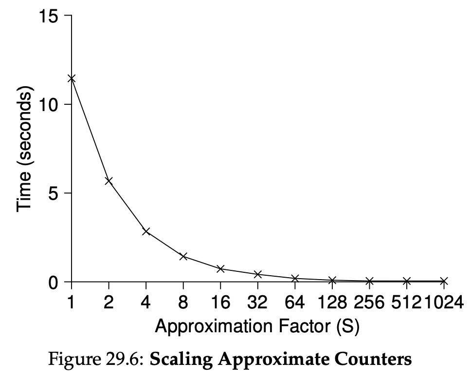
29.2 Concurrent Linked Lists
Scaling Linked Lists
Though we again have a basic concurrent linked list, once again we are in a situation where it does not scale particularly well. One technique that researchers have explored to enable more concurrency within a list is something called hand-over-hand locking(a.k.a. lock coupling). The idea is pretty simple. Instead of having a single lock for the entire list, you instead add a lock per node of the list. When traversing the list, the code first grabs the next node’s lock and then releases the current node’s lock(which inspires the name hand-over-hand). Conceptually, a hand-over-hand linked list makes some sense; it enable a high degree of concurrency in list operations. However, in practice, it is hard to make such a structure faster than the simple single lock approach, as the overheads of acquiring and releasing locks for each node of a list traversal is prohibitive. Even with very large lists, and a large number of threads, the concurrency enable by allowing mutiple ongoing traversals is unlikely to be faster than simply grabbing a single lock, performancing an operation, and releasing it. Perhaps some kind of hybrid(where you grab a new lock every so many nodes) would be worth investigating.
29.3 Concurrent Queues
If you study the code carefully, you’ll notice that there are two locks, one for the head of the queue, and one for the tail. The goal of these two locks is to enable concurrency of enqueue and dequeue operations. In the common case, the enqueue routine will only access the tail lock, and dequeue only the head lock.
29.5 Summary
To be careful with acquisition and release of locks around control flow changes; that enabling more concurrency does not necessarily increase performance; that performance problems should only be remedied once they exist.
The last point, of avoiding premature optimization, is central to any performance-minded developer; there is no value in making something faster if doing so will not improve the overall performance of the application.
30 Condition Variables
30.1 Definition and Routines
To wait for a condition to become true, a thread can make use of what is known as a condition variable. A condition variable is an explicit queue that threads can put themeselves on when some state of execution(i.e., some condition) is not as desired(by waiting on the condition); some other thread, when it changes said state, can then wake one(or more) of those waiting threads and thus allow them to continue(by signaling on the condition).
One thing you might notice about the wait() call is that it also takes a mutex as a parameter; it assumes that this mutex is locked when wait() is called. The responsibilities of wait() is to release the lock and put the calling thread to sleep(atomically); when the thread wakes up(after some other thread has signaled it), it must re-acquire the lock before returning to the caller.
30.2 The Producer/Consumer(Bounded Buffer) Problem
Imagine one or more producer threads and one or more consumer threads. Producers generate data items and place them in a buffer; consumers grab said items from the buffer and consume them in the some way.
The single Buffer Producer/Consumer Solution
Using two condition variables, instead of one, in order to properly signal which type of thread should wake up when the state of the system changes.
TIP: USE WHILE(NOT IF) FOR CONDITION When checking for a condition in a multi-threaded program, using a while loop is always correct; using an if statement only might be, depending on the semantics of signaling. Thus, always using while and your code will behave as expected. Using while loops around conditional checks also handles the case where spurious wakeup occur.
31 Semaphores
31.1 Semaphores: A Definition
A semaphore is an object with an integer value that we can manipulate with two routines.
31.2 Binary Semaphores(Locks)
Because locks only have two states(held and not held), we sometimes call a semaphore used as a lock a binary semaphore.
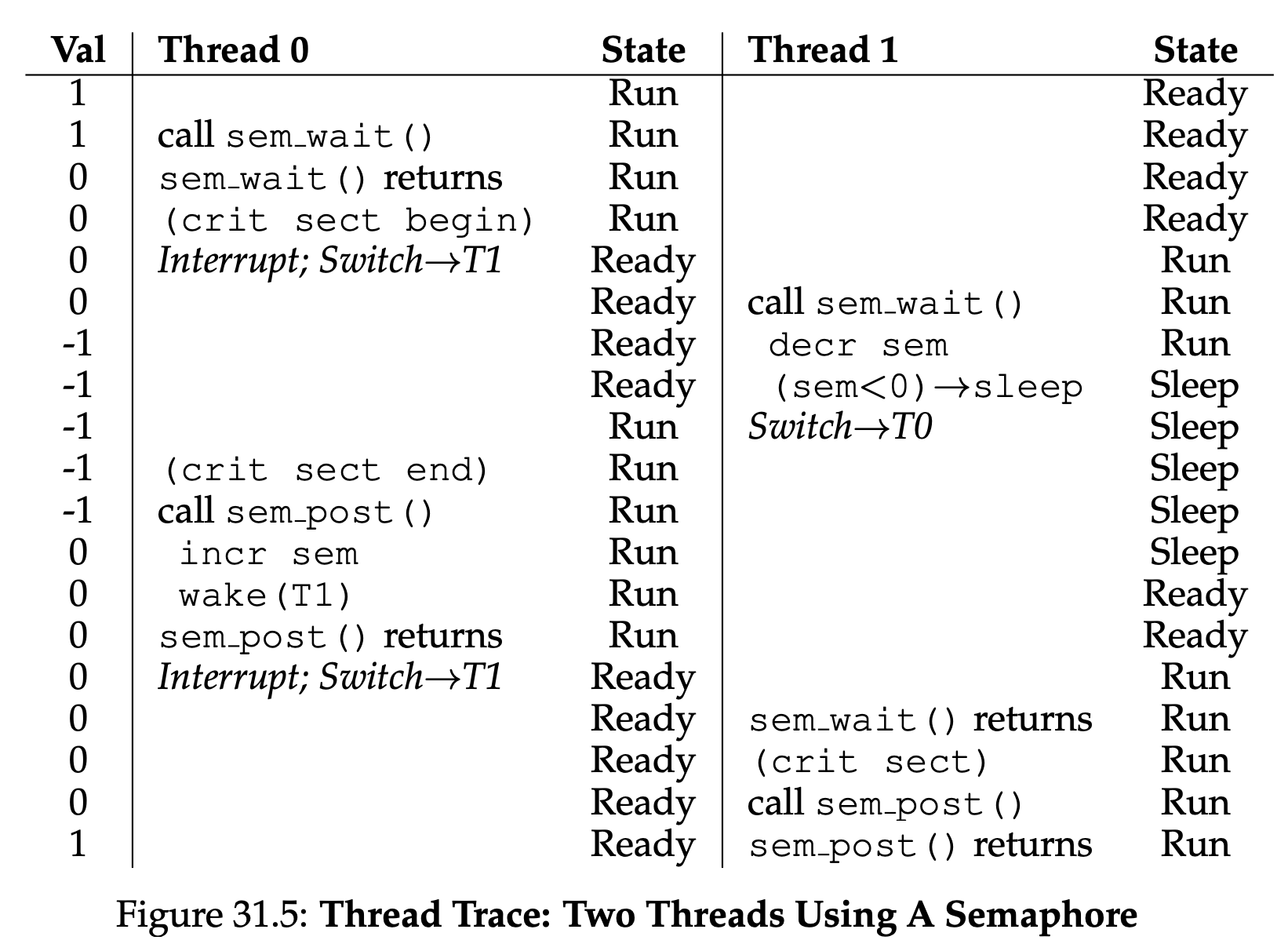
31.3 Semaphores For Ordering
In this pattern of usage, we often find one thread waiting for something to happen, and another thread making that something happen and then signaling that it has happened, thus waking the waiting thread. We are thus using the semaphore as an ordering primitive(similar to our use of condition variables eariler).
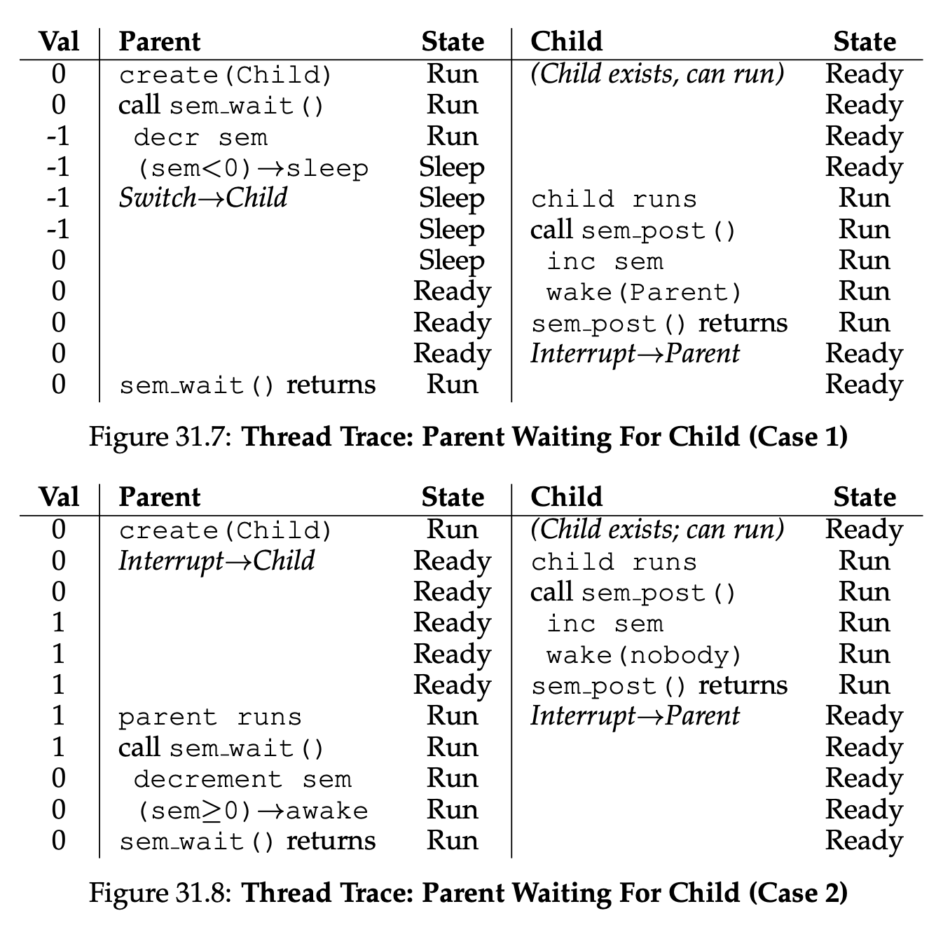
With the lock, it was 1, because you are willing to have the lock locked(given away) immediately after initialization. With the ordering case, it was 0, because there is nothing to give away at the start.
31.6 The Dining Philosophers
The basic setup for the problem is this(as shown in Figure 31.14): assume there are five “philosophers” sitting around a table. Between each pair of philosophers is a single fork(and thus, five total). The pholosphers each have times where they think, and don’t need any forks, and times where they eat. In order to eat, a philosopher needs two forks, both the one on their left and the one on the right.
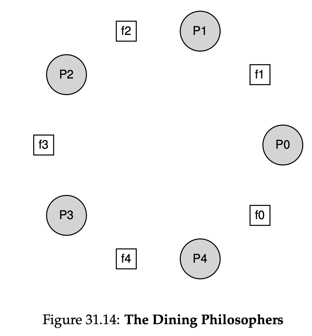
Broken Solution
To acquire the forks, we simply grab a “lock” on each one: first the one on the left, and then the one on the right. When we are done eating, we release them. There is a deadlock problem. If each philosopher happens to grab the fork on their left before any pholospher can grab the fork on their right, each will be stuck holding one fork and waiting for another, forever.
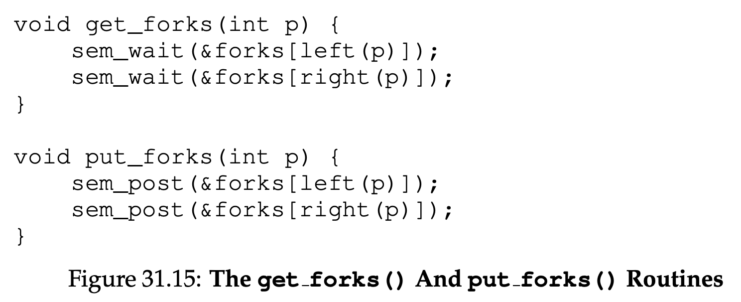
A solution: Breaking The Dependency
Let’s assume that philosopher 4(the highest numbered one) gets the forks in a different order than the others; the put_forks() code remains the same. Because the last philosopher tries to grab right before left, there is no situation where each philosopher grabs one fork and is stuck waiting for another; the cycle of waiting is broken.
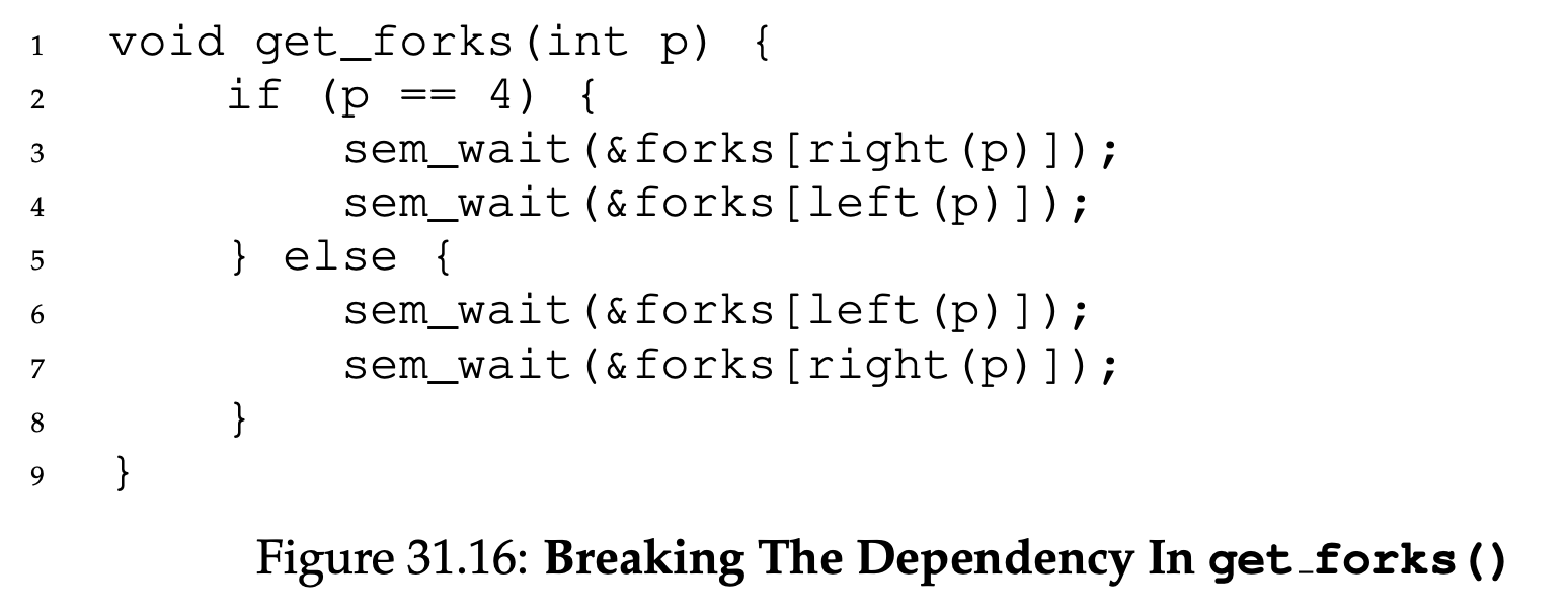
31.7 Thread Throttling
The specific problem is this: how can a programmer prevent “too many” threads from doing something at once and bogging the system down? Answer: decide upon a threshold for “too many”, and then use a semaphore to limit the number of threads concurrently executing the piece of code in question. We call this approach throttling, and consider it a form of admission control.
Imagine that you create hundreds of threads to work on some problem in parallel. However, in a certain part of the code, each thread acquires a large amount of memory to perform part of the computation; let’s call this part of the code the memory-intensive region. If all of the threads enter the memory-intensive region at the same time, the sum of all the memory allocation requests will exceed the amount of physical memory on the machine. As a result, the machine will start thrashing(i.e., swapping pages to and from the disk), and the entire computation will slow to a crawl.
A simple semaphore can solve this problem. By initializing the value of the semaphore to the maximum number of threads you wish to enter the memory-intensive region at once, and then putting a sem_wait() and sem_post() around the region, a semaphore can naturally throttle the number of threads that are ever concurrently in the dangerous region of the code.
32 Common Concurrency Problems
32.2 Non-Deadlock Bugs
Atomicity-Violation Bugs
The desired serializability among multiple memory accesses is violated(i.e. a code region is intended to be atomic, but the atomicity is not enforced during execution).
Order-Violation Bugs
The disired order between two(groups of) memory accesses if flipped(i.e., A should always be executed before B, but the order is not enforced during execution)
32.3 Deadlock Bugs
Deadlock occurs, for example, when a thread(say Thread 1) is holding a lock(L1) and waiting for another one(L2); unfortunately, the thread(Thread 2)that holds lock L2 is waiting for L1 to be released.
Note that if this code runs, deadlock does not necessarily occur; rather, it may occur, if, for example, Thread 1 grabs lock L1 and then a context switch occurs to Thread 2. At that point, Thread 2 grabs L2, and tries to acquire L1. Thus we have a deadlock, as each thread is waiting for the other and neither can run.
Conditions for Deadlock
Four conditions need to hold for a deadlock to occur:
- Mutual exclusion: Threads claim exclusive control of resources that they require(e.g., a thread grabs a lock)
- Hold-and-wait: Threads hold resources allocated to them(e.g., locks that they have already acquired) while waiting for additional resources(e.g., locks that they wish to acquire).
- No preemption: Resources(e.g., locks) cannot be forcibly removed from threads that are holding them.
- Circular wait: There exists a circular chain of threads such that each thread holds one or more resources(e.g., locks) that are being requested by the next thread in the chain. If any of these four conditions are not met, deadlock cannot occur.
Prevention
Circular Wait
The most straightforward way to do that is to provide a total ordering on lock acquisition. For example, if there are only two locks in the system(L1 and L2), you can prevent deadlock by always acquiring L1 before L2. Such strict ordering ensures that no cyclical wait arises; hence, no deadlock. Of course, in more complex systems, more than two locks will exist, and thus total lock ordering may be difficult to achieve. Thus, a partial ordering can be a useful way to structure lock acquisition so as to avoid deadlock.
Hold-and-wait
The hold-and-wait requirement for deadlock can be avoided by acquiring all locks at once, atomically.
No Preemption
Because we generally view locks as held until unlock is called, multiple lock acquisition often gets us into trouble because when waiting for one lock we are holding another. Many thread libraries provide a more flexible set of interfaces to help avoid this situaion. Specifically, the routine pthread_mutex_trylock() either grabs the lock(if it is available) and returns success or returns an error code indicating the lock is held; in the latter case, you can try again later if you want to grab that lock.
top:
  pthread_mutex_lock(L1);
  if(pthread_mutex_trylock(L2) != 0){
       pthread_mutex_unlock(L1);
       goto top;
}
Note that another thread could follow the same protocol but grab the locks in the other order(L2 then L1) and the program would still be deadlock free. One new problem does arise, however: livelock. It is possible (though perhaps unlikely) that two threads could both be repeatedly attempting this sequence and repeatedly failing to acquire both locks. In this case, both systems are running through this code sequence over and over again(and thus it is not a deadlock), but progress is not being made, hence the name livelock. There are solutions to the livelock problem, too: for example, one could add a random delay before looping back and trying the entire thing over again, thus decreasing the odds of repeated interference among competing threads.
You might also notice that this approach doesn’t really add preemption(the forcible action of taking a lock away from a thread that owns it), but rather uses the trylock approach to allow a developer to back out of lock ownership in a graceful way. However, it is a practical approach, and thus we include it here, despite its imperfection in this regard.
Mutual Excluion
The final prevention technique would be to avoid the need for mutual exclusion at all. The idea behind these lock-free(and related wait-free) approaches here is simple: using powerful hardware instructions, you can build data structures in a manner that does not require explicit locking.
Let’s consider a slightly more complex exampel: list insertion. Here is code that inserts at the head of a list:
void insert(int value){
   node_t *n = malloc(sizeof(node_t));
   assert(n != NULL);
   n->value = value;
   n->next = head;
   head = n;
}
This code performs a simple insertion, but if called by multiple threads at the “same time”, has a race condition. We could solve this by surrounding this code with a lock acquire and release:
void insert(int value){
   node_t *n = malloc(sizeof(node_t));
   assert(n != NULL);
   n->value = value;
   pthread_mutex_lock(list_lock);  // begin critical section
   n->next = head;
   head = n;
   pthread_mutex_unlock(listlock); // end critical section
}
In this solution, we are using locks in the traditional manner. Instead, let us try to perform this insertion in a lock-free manner simply using the compare-and-swap instruction. Here is one possible approach:
void insert(int value){
   node_t *n = malloc(sizeof(node_t));
   assert(n != NULL);
   n->value = value;
   do{
       n->next = head;
   }while(CompareAndSwap(&head,n->next,n) == 0);
}
The code here updates the next pointer to point to the current head, and then tries to swap the newly-created node into position as the new head of the list. However, this will fail if some other thread successfully swapped in a new head in the meanwhile, causing this thread to retry again with the new thread.
Deadlock Avoiding via Scheduling
Instead of deadlock prevention, in some scenarios deadlock avoidance is preferable. Avoidance requires some global knowledge of which locks various threads might grab during their execution, and subsequently schedules said threads in a way as to guarantee no deadlock can occur.
Though it may have been possible to run these tasks concurrently, the fear of deadlock prevents us from doing so, and the cost is performance. Unfortunately, they are only useful in very limited environments, for example, in an embedded system where one has full knowledge of the entire set of tasks that must be run and the locks that they need. Further, such approaches can limit concurrency. Thus, avoidance of deadlock via scheduling is not a widely-used general-purpose solution.
33 Event-based Concurrency(Advanced)
33.1 The Basic Idea: An Event Loop
The approach is quite simple: you simply wait for something(i.e., an “event”) to occur; when it does, you check what type of event it is and do the small amount of work it requires(which may include issuing I/O requests, or scheduling other events for future handling, etc.).
33.4 Why Simpler? No Locks Needed
With a single CPU and an event-based application, the problems found in concurrent programs are no longer present. Specifically, because only one event is being handled at a time, there is no need to acquire or release locks; the event-based server cannot be interrupted by another thread because it is decidedly single threaded.
33.5 A Problem: Blocking System Calls
With an event-based approach, however, there are no other threads to run: just the main event loop. And this implies that if an event handler issues a call that blocks, the entire server will do just that: block until the call completes. When the event loop blocks, the system sits idle, and thus is a huge potential waste of resources. We thus have a rule that must be obeyed in event-based systems: no blocking calls are allowed.
33.7 Another Problem: State Management
Another issue with the event-based application is that such code is generally more complicated to write than traditional thread-based code. The reason is as follows: when an event handler issues an asynchronous I/O, it must package up some program state for the next event handler to use when the I/O finally completes; this additional work is not needed in thread-based program, as the state the program needs is on the stack of the thread.
The solution would be to record the socket descriptor(sd) in some kind of data structure(e.g., a hash table), indexed by the file descriptor(fd). When the disk I/O completes, the event handler would use the file descriptor to look up the continuation, which will return the value of the socket descriptor to the caller. At this point, the server can then do the last bit of work to write the data to the socket.
36 I/O Device
36.1 System Architecture
The faster a bus is, the shorter is must be; thus, a high-performance memory bus doesn’t have much room to plug devices and such into it. In addition, engineering a bus for high performance is quite costly. Thus, system designers have adopted this hierarchical approach, where components that demand high performance(such as the graphics card) are nearer the CPU. Lower performance components are further away. The benefits of placing disks and other slow devices on a peripheral bus are manifold; in particular, you can place a large number of devices on it.
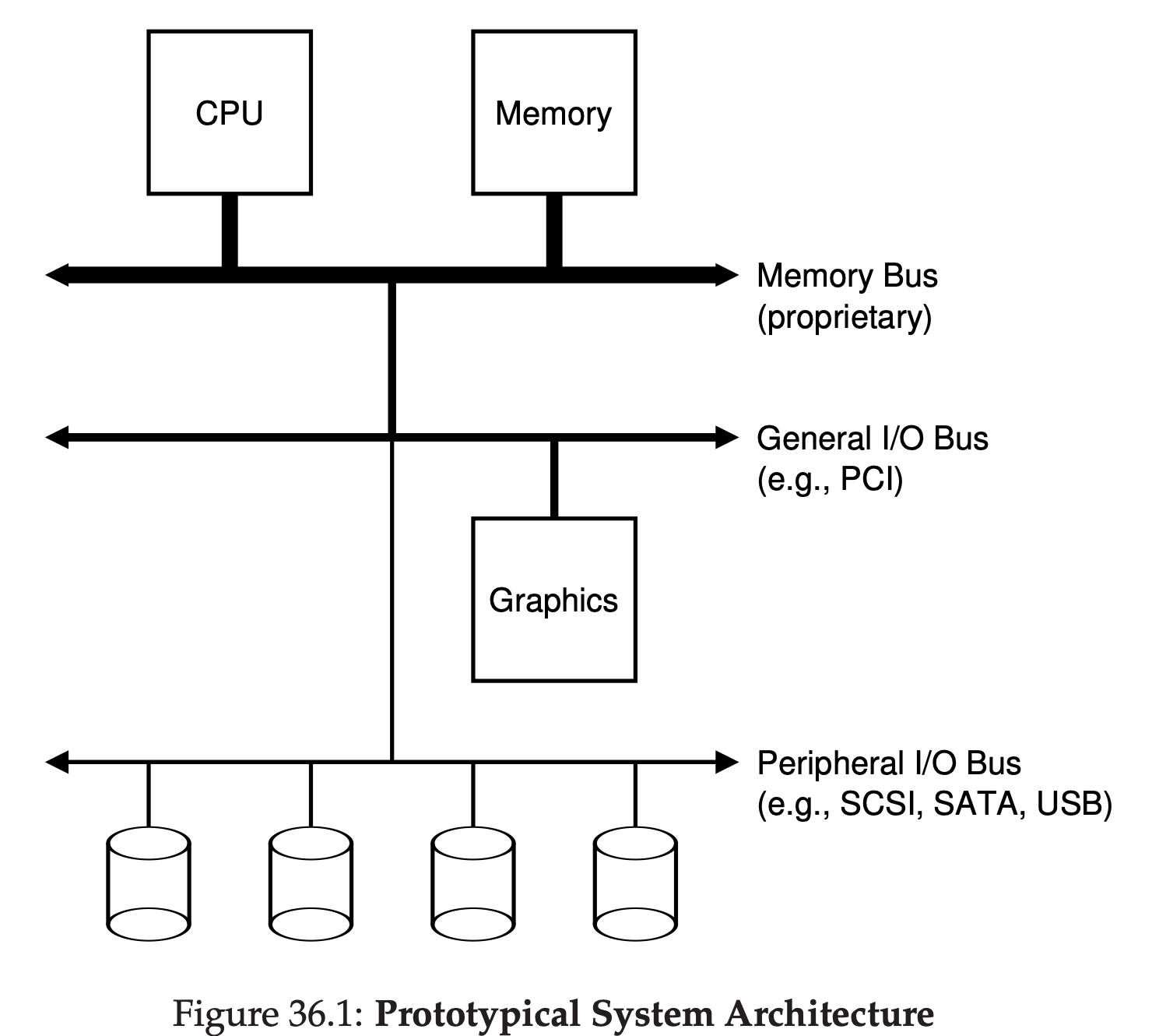
36.2 A Canonical Device
There are two important components. The first is the hardware interface it presents to the rest of the system. Just like a piece of software, hardware must also present some kind of interface that allows the system software to control its operation. Thus, all devices have some specified interface and protocol for typical interaction. The second part of any device is its internal structure. This part of the device is implementation specific and is responsible for implementing the abstraction the device presents to the system.
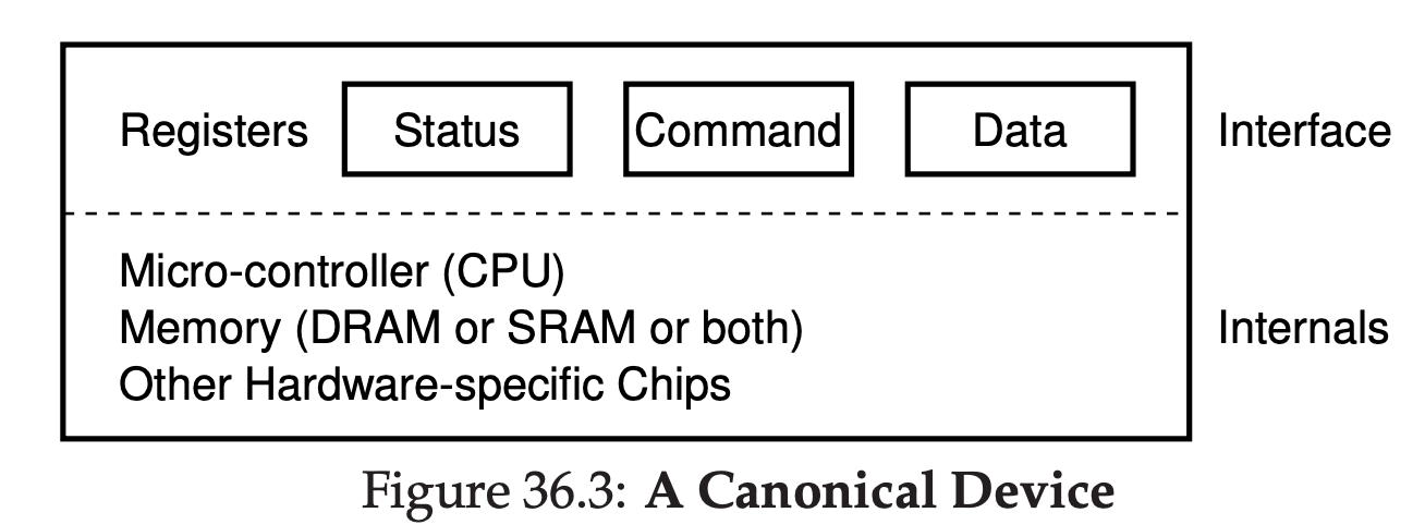
36.3 The Canonical Protocol
In the picture above, the device interface is comprised of three registers: a status register, which can be read to see the current status of the device; a command register, to tell the device to perform a certain task; and a data register to pass data to the device, or get data from the device. By reading and writing these registers, the operating system can control device behavior.
The protocol has four steps. In the first, the OS waits until the device is ready to receive a command by repeatedly reading the status register; we call this polling the device(basically, just asking it what is going on). Second, the OS sends some data down to the data register; one can imagine that if this were a disk, for example, that multiple writes would need to take place to transfer a disk block to the device. When the main CPU is involved with the data movement, we refer to it as programmed I/O(PIO). Third, the OS writes a command to the command register; doing so implicitly lets the device know that both the data is present and that it should begin working on the command. Finally, the OS waits for the device to finish by again polling it in a loop, waiting to see if it is finished(it may then get an error code to indicate success or failure).
while(STATUS == BUSY)
   ; // wait until device is not busy
write data to DATA register
write command to COMMAND register
   (starts the device and executes the command)
while(STATUS == BUSY)
   ; // wait until device is done with your request
36.4 Lowering CPU overhead With interrupts
Instead of polling the device repeatedly, the OS can issue a request, put the calling process to sleep, and context switch to another task. When the device if finally finished with the operation, it will raise a hardware interrupt, causing the CPU to jump into the OS at a predetermined interrupt service routine(ISR) or more simply an interrupt handler. The handler is just a piece of operating system code that will finish the request and wake the process waiting for the I/O, which can then proceed as desired.
Note that using interrupts is not always the best solution. For example, imagine a device that performs its tasks very quickly: the first poll usually finds the device to be done with task. Using an interrupt in this case will actually slow down the system: switching to another process, handling the interrupt, and switching back to the issuing process is expensive. Thus, if a device is fast, it may be best to poll; if it is slow, interrupts, which allow overlap, are best. If the speed of the device is not known, or sometimes fast and sometimes slow, it may be best to use a hybrid that polls for a little while and then, if the device is not yet finished, uses interrupts. This two-phased approach may achieve the best of both worlds.
36.5 More Efficient Data Movement With DMA
When using programmed I/O(PIO) to transfer a large chunk of data to a device, the CPU is once again overburdened with a rather trivial task, and thus wastes a lot of time and effort that could better be spent running other processes. The solution to this problem is something we refer to as Direct Memorg Access(DMA). A DMA engine is essentially a very specific device within a system that can orchestrate transfers between devices and main memory without much CPU intervention.
36.6 Methods Of Device Interaction
The first, oldest method is to have explicit I/O instructions. These instructions specify a way for the OS to send data to specify device registers and thus allow the construction of the protocols described above. The second method to interact with devices is known as memory-mapped I/O. With this approach, the hardware makes device registers available as if they were memory locations. To access a particular register, the OS issues a load(to read) or store(to write) the address; the hardware then routes the load/store to the device instead of main memory.
36.7 Fitting Into The OS: The Device Driver
How to fit devices, each of which have very specific interfaces, into the OS, which we would like to keep as general as possible. The problem is solved through the age-old technique of abstraction. At the lowest level, a piece of software in the OS must know in detail how a device works. We call this piece of software a device driver, and any specifics of device interaction are encapsulated within.
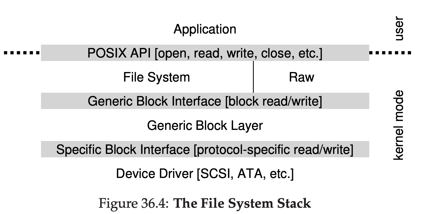
Note that the encapsulation seen above can have its downside as well. If there is a device that has many special capabilities, but has to present a generic interface to the rest of the kernel, those special capabilities will go unused.
Interestingly, because device drivers are needed for any device you might plug into your system, over time they have come to represent a huge percentage of kernel code. Studies of the Linux kernel reveal that over 70% of OS code is found in device drivers; for Windows-based systems; it is likely quite high as well.
37 Hard Disk Drives
37.1 The Interface
The drive consists of a large number of sectors(512-byte blocks), each of which can be read or written. The sectors are numbered from 0 to n-1 on a disk with n sectors. Thus, we can view the disk as an array of sectors; 0 to n-1 is thus the address space of the drive.
Multi-sector operations are possible; indeed, many file systems will read or write 4KB at a time(or more). However, when updating the disk, the only guarantee drive manufacturers make is that a single 512-byte write is atomic; thus, if an untimely power loss occurs, only a portion of a larger write may complete(sometimes called a torn write).
37.2 Basic Geometry
We start with a platter, a circular hard surface on which data is stored persistently by inducing magnetic changes to it. A disk may have one or more platter; each platter has 2 sides, each of which is called a surface. These platters are usually made of some hard material(such as aluminum), and then coated with a thin magnetic layer that enables the drive to persistently store bits even when the drive is powered off.
The platters are all bound together around the spindle, which is connected to a motor that spins the platters around at a constant rate.
Data is encoded on each surface in concentric circule of sectors; we call one such concentric circle a track.
To read and write from the surface, we need a mechanism that allows us to either sense(i.e., read) the magnetic patterns on the disk or to induce a change in(i.e., write) them. This process of reading and writing is accomplished by the disk head; there is one such head per surface of the drive. The disk head is attached to a single disk arm, which moves across the surface to position the head over the desired track.
37.3 A Simple Disk Drive
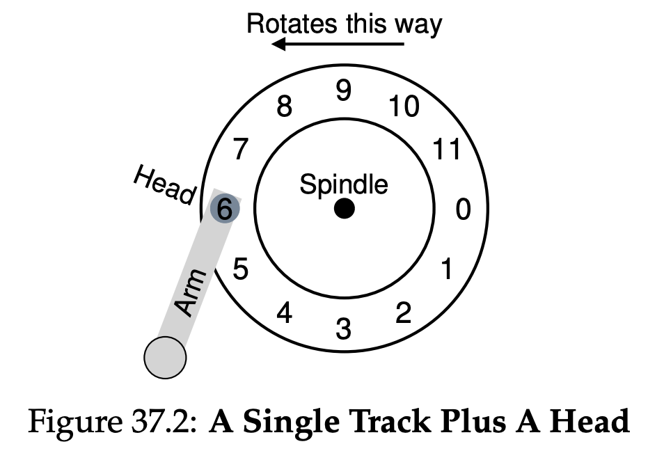
Single-track Latency: The Rotational Delay
Imagine we now receive a request to read block 0. The disk doesn’t have to do much. In particular, it must just wait for the desired sector to rotate under the disk head. This wait happens often enough in modern drives, and is an important enough component of I/O service time, that it has a special name: rotational delay.
Multiple Tracks: Seek Time
A read to sector 11. To service this read, the drive has to first move the disk arm to the correct track(in this case, the outermost one), in a process known as a seek. Seeks, along with roataions, are one of the most costly disk operations. During the seek, the arm has been moved to the desired track, and the platter of course has rotated, in this case about 3 sectors. Thus, sector 9 is just about to pass under the disk head, and we must only endure a short rotational delay to complete the transfer. When sector 11 passes under the disk head, the final phase of I/O will take place, known as the transfer, where data is either read from or write to the surface. And thus, we have a complete picture of I/O time: first a seek, then waiting for the rotational delay, and finally the transfer.
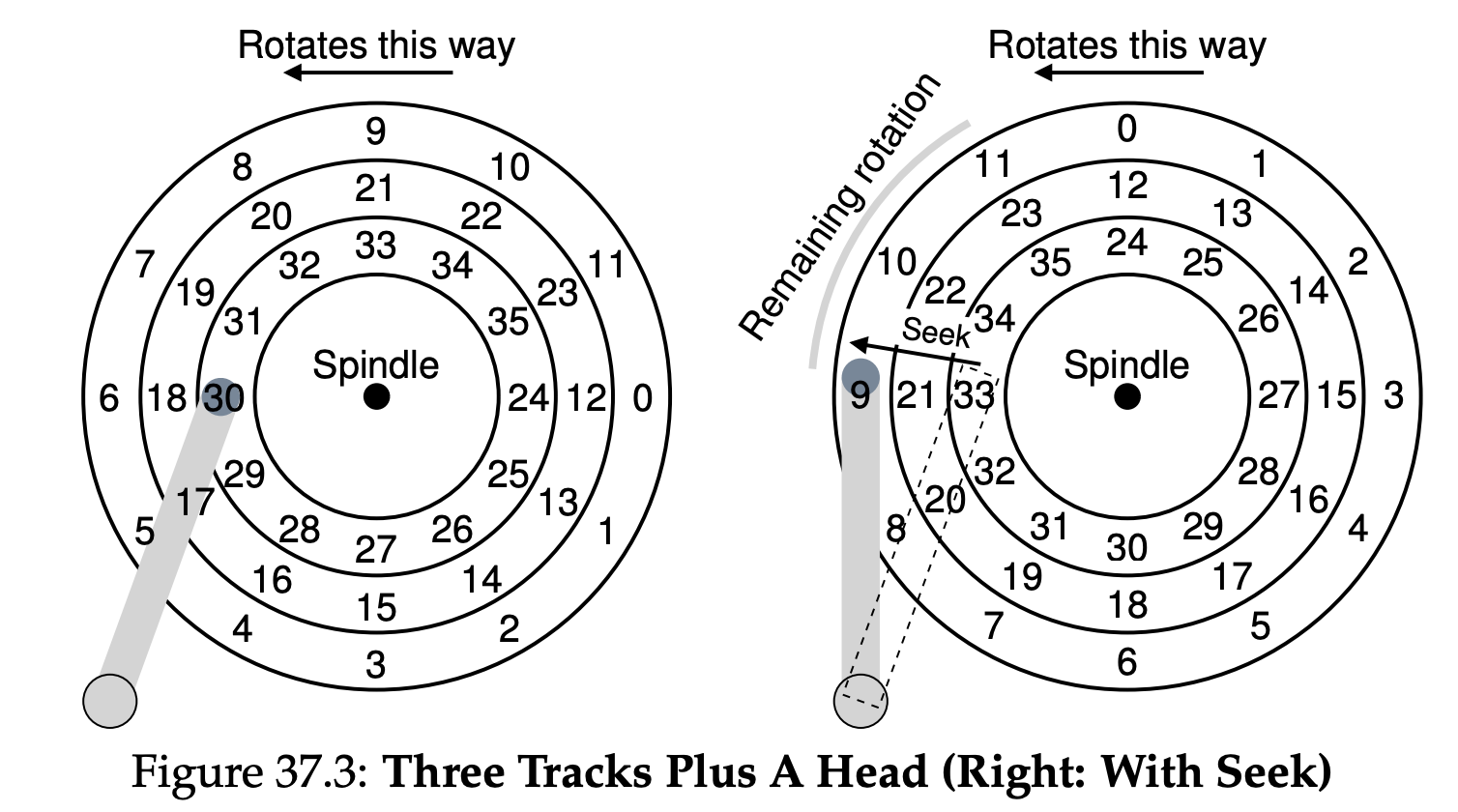
37.4 I/O Time: Doing The Math
We can now represent I/O time as the sum of three major components: $T_{I/O}$ = $T_{Seek}$ + $T_{Rotation}$ + $T_{Transfer}$ Note that the rate of I/O($R_{I/O}$) is easily computed from the time. Simply divide the size of the transfer by the time it took: $R_{I/O}$ = $\frac{Size_{Transfer}}{T_{I/O}}$
The first is the “high performance” drive market, where drives are engineered to spin as fast as possible, deliver low seek times, and transfer data quickly. The second is the “capacity” market, where cost per byte is the most important aspect; thus the drives are slower but pack as many bits as possible into the space available.
37.5 Disk Scheduling
Given a set of I/O requests, the disk scheduler examines the requests and decides which one to schedule next.
Unlike job scheduling, we can make a good guess at how long a “job”(i.e., disk request) will take. By estimating the seek and possible rotational delay of a request, the disk scheduler can know how long each request will take, and thus(greedily) pick the one that will take the least time to service first.
SSFT: Shortest Seek Time First
SSFT orders the queue of I/O requests by track, picking requests on the nearest track to complete first.
There is a starvation problem. Imagine that there were a steady stream of requests to the inner track, where the head currently is positioned. Requests to any other tracks would then be ignored completely by a pure SSTF approach.
Elevator(a.k.a. SCAN or C-SCAN)
SCAN simply moves back and forth across the disk servicing requests in order across the tracks. Let’s call a single pass across the disk a sweep. If a request comes for a block on a track that has already been serviced on this sweep of the disk, it is not handled immediately, but rather queued until the next sweep.
Unfortunately, SCAN and its cousins do not represent the best scheduling technology. In particular, SCAN does not actually adhere as closely to the principle of SJF as they could. In particular, they ignore rotation.
38 Redundant Arrays of Inexpensive Disks(RAIDs)
Externally, a RAID looks like a disk: a group of blocks one can read or write. Internally, the RAID is a complex beast, consisting of multiple disks, memory, and one or more processors to manage the system. A hardware RAID is very much like a computer system, specialized for the task of managing a group of disks.
RAIDs offer number of advantages over a single disk. One advantage is performance. Using multiple disks in parallel can greatly speed up I/O times. Another benefit is capacity. Large data sets demand large disks. Finally, RAIDs can improve reliability; spreading data across multiple disks(without RAID techniques) makes the data vulnerable to the loss of a single disk; with some form of redundancy, RAIDs can tolerate the loss of a disk and keep operating as if nothing were wrong.
38.1 Interface And RAID Internals
To a file system above, a RAID looks like a big,(hopefully) fast, and (hopefully) reliable disk. Just as with a single disk, it presents itself as a linear array of blocks, each of which can be read or written by the file system(or other client).
When a file system issues a logical I/O request to the RAID, the RAID internally must calculate which disk(or disks) to access in order to complete the request, and then issue one or more physical I/Os to do so. The exact nature of these physical I/Os depends on the RAID level, as we will discuss in detail below. However, as a simple example, consider a RAID that keeps two copies of each block(each one on a separate disk); when writing to such a mirrored RAID system, the RAID will have to perform two physical I/Os for every one logical I/O it is issued.
At a high level, a RAID is very much a specialized computer system: it has a processor, memory, and disks; however, instead of running applications, it runs specialized software designed to operate the RAID.
38.3 How To Evaluate A RAID
- The first axis is capacity;
- The second axis of evaluation is reliability.
- The third axis is performance.
38.4 RAID Level 0: Striping
The first RAID level is actually not a RAID level at all, in that there is no redundancy.
From Figure 38.1, you get the basic idea: spread the blocks of the array across th disks in a round-robin fashion. This approach is designed to extract the most parallelism from the array when request are made for contiguous chunks of the array(as in a large, sequential read, for example). We call the blocks in the same row a stripe; thus, blocks 0,1,2, and 3 are in the same stripe.
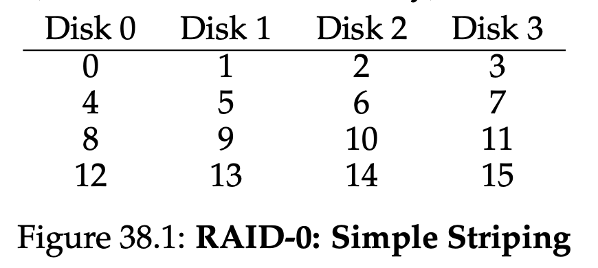
Chunk Sizes
Chunk size mostly affects performance of the array, For example, a small chunk size implies that many files will get striped across many disks, thus increasing the parallelism of reads and writes to a single file; however, the positioning time to access blocks across mutliple disks increases, because the positioning time for the entire request is determined by the maximum of the positioning times of the requests across all drives. A big chunk size, on the other hand, reduces such intra-file parallelism, and thus relies on mulitple concurrent requests to achieve high throughput. However, large chunk size reduce positioning time; if, for example, a single file fits within a chunk and thus is placed on a single disk, the positioning time incurred while accessing it will just be the positioning time of single disk.
Back To RAID-0 Analysis
From the perspective of capacity, it is perfect: given N disks each of size B blocks, striping delievers N·B blocks of useful capacity. From the standpoint of reliability, striping is also perfect, but in the bad news: any disk failure will lead to data loss. Finally, performance is excellent: all disks are utilized, often in parallel, to service user I/O requests.
Evaluating RAID Performance
The first is single-request latancy. Understanding the latency of a single I/O request to a RAID is useful as it reveals how much parallelism can exist during a single logical I/O operation. The second is steady-state throughput of the RAID, i.e., the bandwidth of many concurrent requests. Because RAIDs are often used in high-performance environments, the steady-state bandwidth is critical, and thus will be the main focus of our analyses.
With sequential access, a disk operates in its most efficient mode, spending little time seeking and waiting for rotation and most of its time transferring data. With random access, just the opposite is true: most time is spent seeking and waiting for rotation and relatively little time is spent transferring data.
38.5 RAID Level 1: Mirroring
With a mirrored system, we simply make more than one copy of each block in the system; each copy should be placed on a separate disk, of course. By doing so, we can tolerate disk failures. In a typical mirrored system, we will assume that for each logical block, the RAID keeps two physical copies of it.
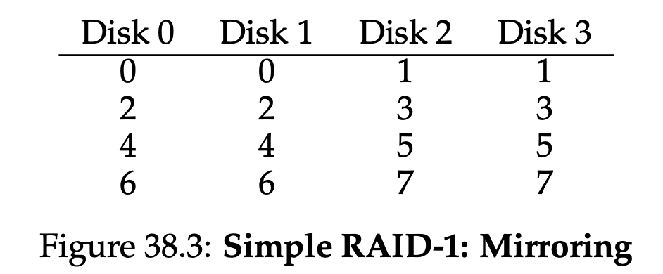
When reading a block from a mirrored array, the RAID has a choice: it can read either copy. For example, if a read to logical block 5 is issued to the RAID, it is free to read it from either disk 2 or disk 3. When writing a block, though, no such choice exists: the RAID must update both copies of the data, in order to preserve reliability. Do note, though, that these writes can take place in parallel; for example, a write to logical block 5 could proceed to disks 2 and 3 at the same time.
RAID-1 Analysis
From a capacity standpoint, RAID-1 is expensive; with the mirroring level = 2, we only obtain half of our peak useful capacity. From a reliability standpoint, RAID-1 does well. It can tolerate the failure of any one disk. From the perspective of the latency of a single read request, we can see it is the same as the latency on a single disk; all the RAID-1 does is direct the read to one of its copies. A write is a little different: it requires two physical writes to complete before it is done.
Using a write-ahead log of some kind to first record what the RAID is about to do before doing it. By taking this approach, we can ensure that in the presence of a crash, the right thing will happen; by running a recovery procedure that replays all pending transactions to the RAID, we can ensure that no two mirrored copies are out of sync. Because logging to disk on every write is probhibitively expensive, most RAID hardware includes a small amount of non-volatile RAM(e.g., battery-backed) where it performs this type of logging.
38.6 RAID Level 4: Saving Space With Parity
Parity-based approaches attempt to use less capacity and thus overcome the huge space penalty paid by mirrored systems. They do so at a cost, however: performance.
For each stripe of data, we have added a single parity block that stores the redundant information for that stripe of blocks.
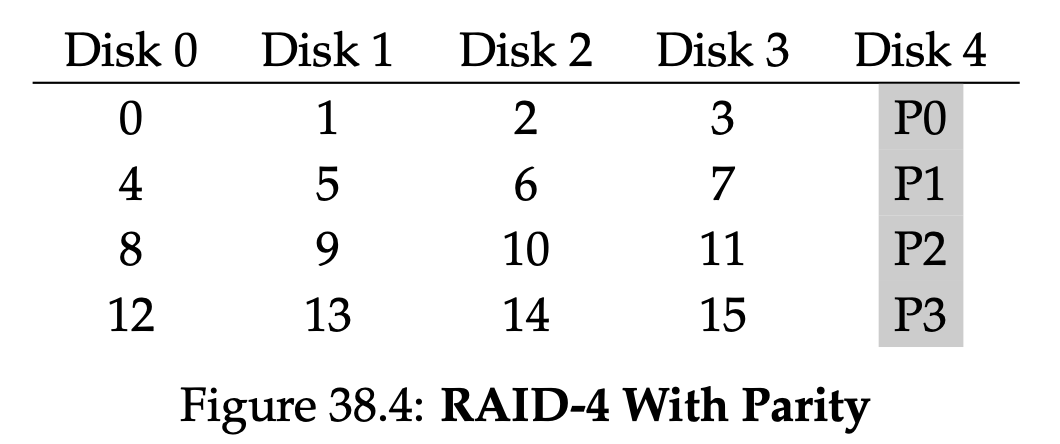
RAID-4 Analysis
From a capacity standpoint, RAID-4 uses 1 disk for parity information for every group of disks it is protecting. RAID-4 tolerates 1 disk failure and no more. If more than one disk is lost, there is simply no way to reconstruct the lost data.
38.7 RAID Level 5: Rotating Parity
RAID-5 works almost identically to RAID-4, except that it rotates the parity block across drives. As you can see, the parity block for each stripe is now rotated across the disks, in order to remove the parity-disk bottleneck for RAID-4.
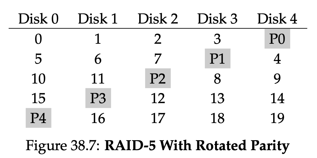
38.8 RAID Comparison: A Summary
To conclude, if you strictly want performance and do not care about reliability, striping is obviously best. If, however, you want random I/O performance and reliability, mirroring is the best; the cost you pay is in lost capacity. If capacity and reliability are your main goals, then RAID-5 is the winner; the cost you pay is in small-write performance. Finally, if you always doing sequential I/O and want to maximum capacity, RAID-5 also makes the most sense.
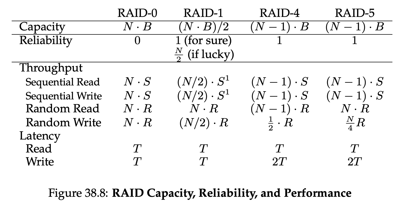
39 Interlude: Files and Directories
Unlike memory, whose contents are lost when there is a power loss, a persistent-storage device keeps such data intact. Thus, the OS must take extra care with such a device: this is where users keep data that they really care about.
39.1 Files And Directories
Two key abstraction have developed over time in the virtualization of storage. The first is the file. A file is simply a linear array of bytes, each of which you can read or write.
In most system, the OS does not know much about the structure of the file(e.g., whether it is a picture, or a text file, or C code); rather, the responsibility of the file system is simply to store such data persistently on disk and make sure that when you request the data again, you get what you put there in the first place.
The second abstraction is that of a directory. A directory, like a file, also has a low-level name(i.e., an inode number), but its contents are quite specific: it contains a list of (user-readable name, low-level name) pairs.
In UNIX systems, the file system thus provides a unified way to access files on disk, USB stick, CD-ROM, many other devices, and in fact many other things, all located under the single directory tree.
39.3 Creating Files
One important aspect of open() is what it returns: a file descriptor. A file descriptor is just an integer, private per process, and is used in UNIX systems to access files; thus, once a file is opened, you use the file descriptor to read or write the file, assuming you have permission to do so. In this way, a file descriptor is a capability. Another way to think of a file descriptor is as a pointer to an object of type file; once you have such an object, you can call other “methods” to access the file, like read() and write().
File descriptors are managed by the operating system on a per-process basis. This means some kind of simple structure(e.g., an array) is kept in the proc structure on UNIX systems. Here is the relevant piece from the vx6 kernel:
struct proc{
  struct file *ofile[NOFILE]; // Open files
}
A simple array(with a maximum of NOFILE open files) tracks which files are opened on a per-process basis. Each entry of the array is actually just a pointer to a struct file, which will be used to track information about the file being read or written.
39.4 Reading And Writing Files
Here is an example of using strace to figure out what cat is doing:
prompt> strace cat foo
...
open("foo", O_RDONLY|O_LARGEFILE) = 3
read(3, "hello\n", 4096) = 6
write(1, "hello\n", 6) = 6
hello
read(3, "", 4096) = 0
close(3) = 0
...
prompt>
The first thing that cat does is open the file for reading. First, the file is only opened for reading(not writing), as indicated by the O_RDONLY flag; second, that the 64-bit offset be used(O_LARGEFILE); third, that the call to open() succeeds and returns a file descriptor, which has the value of 3. Why does the first call to open() return 3, not 0 or perhaps 1 as you might expect? As it turns out, each running process already has three files open, standard input(which the process can read to receive input), standard output(which the process can write to in order to dump information to the screen), and standard error( which the process can write error message to). There are represented by file descriptors 0,1 and 2, respectively. Thus, when you first open another file(as cat does above), it will almost certainly be file descriptor 3.
Each process maintains an array of file descriptors, each of which refers to an entry in the system-wide open file table. Each entry in this table tracks which underlying file the descriptor refer to, the current offset, and other relevant details such as whether the file is readable or writable.
39.5 Reading And Writing, But Not Sequentially
Let’s track a process that opens a file(of size 300 bytes) and reads it by calling the read() system call repeatedly, each time reading 100 bytes. Here is a trace of the relevant system calls, along with the values returned by each system call, and the value of the current offset in the open file table for this file access:
There are a couple of items of interest to note from the trace. First, you can see how the current offset gets initialized to zero when the file is opened. Next, you can see how it is incremented with each read() by the process; this makes it easy for a process to just keep calling read() to get the next chunk of the file. Finally, you can see how at the end, an attempted read() past the end of the file returns zero, thus indicating to the process that it has read the file in its entirety.
Let’s trace a process that opens the same file twice and issue a read to each of them.
In this example, two file descriptors are allocated(3 and 4), and each refers to a different entry in the open file table(in this example, entries 10 and 11, as shown in the table heading, OFT stands for open file table).
A process uses lseek() to reposition the current offset before reading; in this case, only a single open file table entry is needed.
Here, the lseek() call first sets the current offset to 200. The subsequent read() then reads the next 50 bytes, and updates the current offset accordingly.
39.6 Shared File Table Entries: fork() And dup()
If some other process reads the same file at the same time, each will have its own entry in the open file table. In this way, each logical reading or writing of a file is independent, and each has its own current offset while it accesses the given file.
Figure 39.3 shows the relationships that connect each process’s private descriptor array, the shared open file table entry, and the reference from it to the underlying file-system inode. Note that we finally make use of the reference count here. When a file table entry is shared, its reference count is incremented; only when both processes close the file(or exit) will the entry be removed.
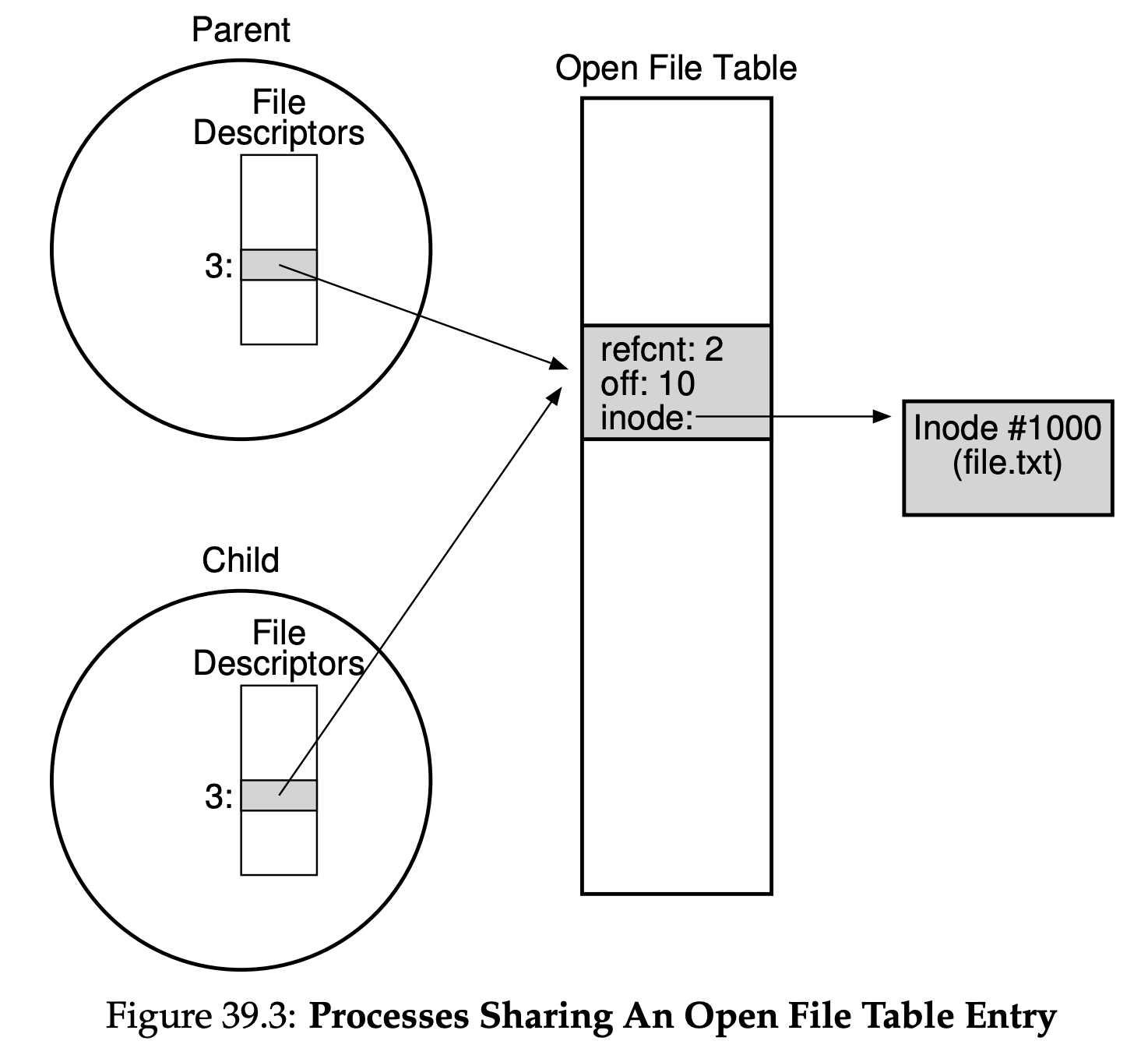
The dup() call allows a process to create a new file descriptor that refers to the same underlying open file as an existing descriptor.
39.7 Writing Immediately With fsync()
Most times when a program calls write(), it is just telling the file system: please write this data to persistent storage, at some point in the future. The file system, for performance reasons, will buffer such writes in memory for some time; at that later point in time, the write(s) will actually be issued to the storage device. However, some applications require something more than this eventual guarantee. When a process calls fsync() for a particular file descriptor, the file system responds by forcing all dirty(i.e., not yet written) data to disk, for the file referred to by the specified file descriptor. The fsync() routine returns once all of those writes are complete.
39.8 Remaing Files
One interesting guarantee provided by the rename() call is that it is (usually) implemented as an atomic call with respect to system crashes; if the system crashes during the remaing, the file will either be named the old name or the new name, and no odd in-between state can arise.
int fd = open("foo.txt.tmp", O_WRONLY|O_CREAT|O_TRUNC,
S_IRUSR|S_IWUSR);
write(fd, buffer, size); // write out new version of file
fsync(fd);
close(fd);
rename("foo.txt.tmp", "foo.txt");
39.9 Getting Information About Files
Beyond file access, we expect the file system to keep a fair amount of information about each file it is storing. We generally call such data about metadata.
39.11 Making Directories
Beyond files, a set of directory-related system calls enable you to make, read, and delete directories. Note you can never write to a directory directly. Because the format of the directory is considered file system metadata, the file system considers itself responsible for the integrity of directory data; thus you can only update a directory indirectly by, for example, creating files, directories, or other object types within it. In this way, the file system makes sure that directory contents are as expected.
39.14 Hard Links
We now come back to the mystery of why removing a file is performed via unlink(), by understanding a new way to make an entry in the file system tree, through a system call known as link().
When you create a file, you are really doing two things. First, you are making a structure(the inode) that will track virtually all relevant information about the file, including its size, where its block are on disk, and so forth. Second, you are linking a human-readable name to that file, and putting that link into a directory. After creating a hard link to a file, to the file system, there is no difference between the original file name and the newly created file name;indeed, they are both just links to the underlying metadata about the file, which is found in the some inode number.
prompt> echo hello > file
prompt> cat file
hello
prompt> ln file file2
prompt> cat file2
hello

prompt> ls -i file file2
67158084 file
67158084 file2
prompt>

prompt> rm file
removed ‘file’
prompt> cat file2
hello
Thus, to remove a file from the file system, we call unlink(). In the example below, we could for example remove the file named file, and still access the file without difficulty. The reason this works is because when the file system unlinks file, it checks a reference count within the inode number. This reference count(sometimes called the link count) allows the file system to track how many different file names have been linked to this particular inode. When unlink() is called, it removes the “link” between the human-readable name(the file that is being deleted) to the given inode number, and decrements are reference count; only when the reference count reaches zero does the file system also free the inode and related data blocks; and thus truly “delete” the file.
39.15 Symbolic Links
There is one other type of link that is really useful, and it is called a symbolic link or sometimes a soft link. Hard links are somewhat limited: you can’t create one to a directory(for fear that you will create a cycle in the directory tree); you can’t hard link to files in other disk partitions(because inode numbers are only unique within a particular file system, not across file systems).
Creating a soft link looks much the same, and the original file can now be accessed through the file name file as well as the symbolic link name file2. However, beyond this surface similarity, symbolic links are actually quite different from hard links. The first difference is that a symbolic link is actually a file itself, of a different type. We’ve already talked about regular files and directories; symbolic links are a third type the file system knows about.
Finally, because of the way symbolic links are created, they leave the possibility for what is known as a dangling reference:
prompt> echo hello > file
prompt> ln -s file file2
prompt> cat file2
hello
prompt> rm file
prompt> cat file2
cat: file2: No such file or directory
As you can see in this example, quite unlink hard links, removing the original file named file causes the link to point to a pathname that no longer exists.
39.16 Permission Bits And Access Control Lists
The file system also presents a virtual view of a disk, transforming it from a bunch of raw blocks into much more user-friendly files and directories. However, the abstraction is notably different from that of the CPU and memory,in that files are commonly shared among different users and processes and are not(always) private.
40 File System Implementaion
The file system is pure software; unlike our development of CPU and memory virtualization, we will not be adding hardware features to make some aspect of the file system work better.
40.1 The Way To Think
To think about file systems, we usually suggest thinking about two different aspect of them; The first is the data structure of the file system. The second aspect of a file system is its access methods.
40.2 Overall Organization
The file system has to track information about each file. This information is a key piece of metadata, and tracks thing like which data blocks comprise a file, the size of the file, its owner and access rights, access and modify times, and other similar kinds of information. To store this information, file systems usually have a structure called an inode.
We’ll need to reserve some space on the disk for inode table, which simply holds an array of on-disk inodes. Assuming 256 bytes per inode, a 4-KB block can hold 16 inodes, and our file system below contains 80 total inodes, this number represents the maximum number of files we can have in our file system.
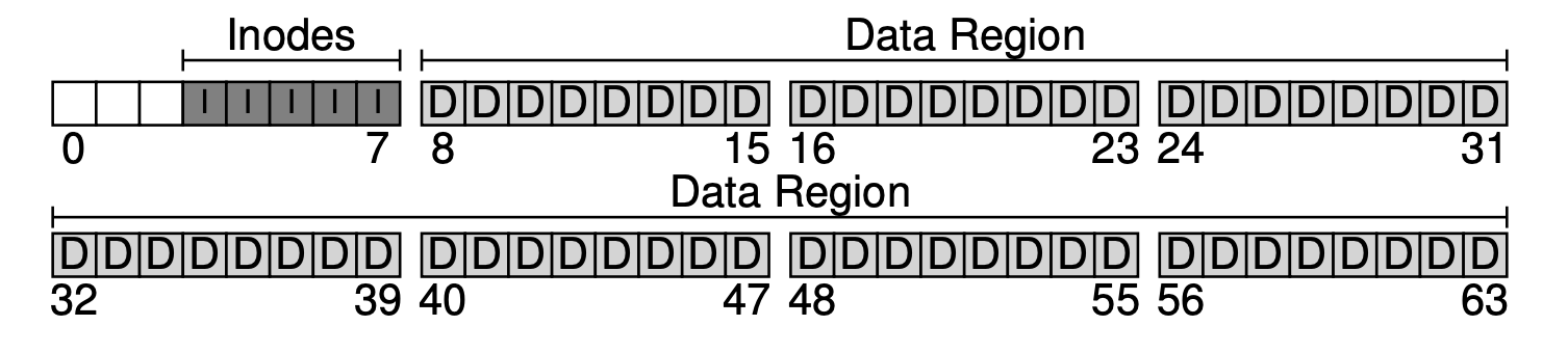
Such allocation structures are thus a requisite element to track whether inodes or data blocks are free or allocated. We choose a simple and popular structure known as a bitmap, one for the data region(the data bitmap), and one for the inode table(the inode bitmap). A bitmap is a simple structure: each bit is used to indicate whether the corresponding object/block is free(0) or in-use(1).
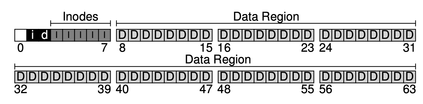
There is one block left in the design of the on-disk structure of our very simple file system. We reserve this for the superblock, denoted by an S in the diagram below. The superblock contains information about this parituclar file system.
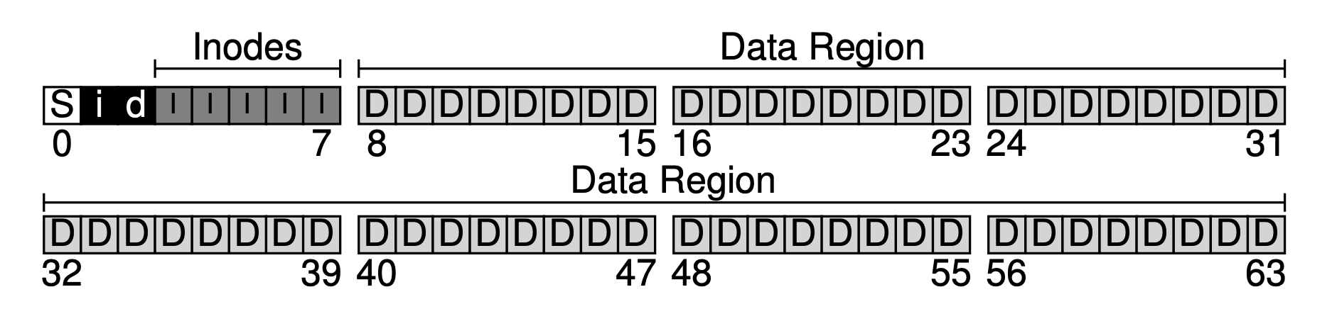
Thus, when mounting a file system, the operating system will read the superblock first, to initialize various parameters, and then attach the volume to the file-system tree. When files within the volume are accessed, the system will thus know exactly where to look for the needed on-disk strutures.
40.3 File Organization: The Inode
One of the most important on-disk structures of a file system is the inode; virtually all file systems have a strucuture similar to this. The name inode is short for index node, the historical name given to it in UNIX and possibly earlier systems, used because these nodes were originally arranged in an array, and the array indexed into when accessing a particular inode.
Each inode is implicitly referred to by a number(called the i-number), which we’ve earlier called the low-level name of the file. For example, take the inode table of vsfs as below: 20KB in size(five 4KB blocks) and thus consisting of 80 inodes(assuming each inode is 256 bytes); further assume that the inode region starts at 12KB(i.e., the superblock starts at 0KB, the inode bitmap is at address 4KB, the data bitmap at 8KB, and thus the inode table comes right after). To read inode number 32, the file system would calculate the offset into the inode region(32 · sizeof(inode) or 8192), add it to the start address of the inode table on disk(inodeStartAddr = 12KB), and thus arrive upon the correct byte address of the desired block of inodes: 20KB.
More generally, the sector address sector of the inode block can be calculated as follows:
blk = (inumber * sizeof(inode_t)) / blockSize;
sector = ((blk * blockSize) + inodeStartAddr) / sectorSize;
Inside each inode is virtually all of the information you need about a file: its type(e.g., regular file, directory, etc.), its size, the number of blocks allocated to it, protection information(such as who owns the file, as well as who can access it), some time information, including when the file was created, modified, or last accessed, as well as information about where its data blocks reside on disk(e.g., pointers of some kind).
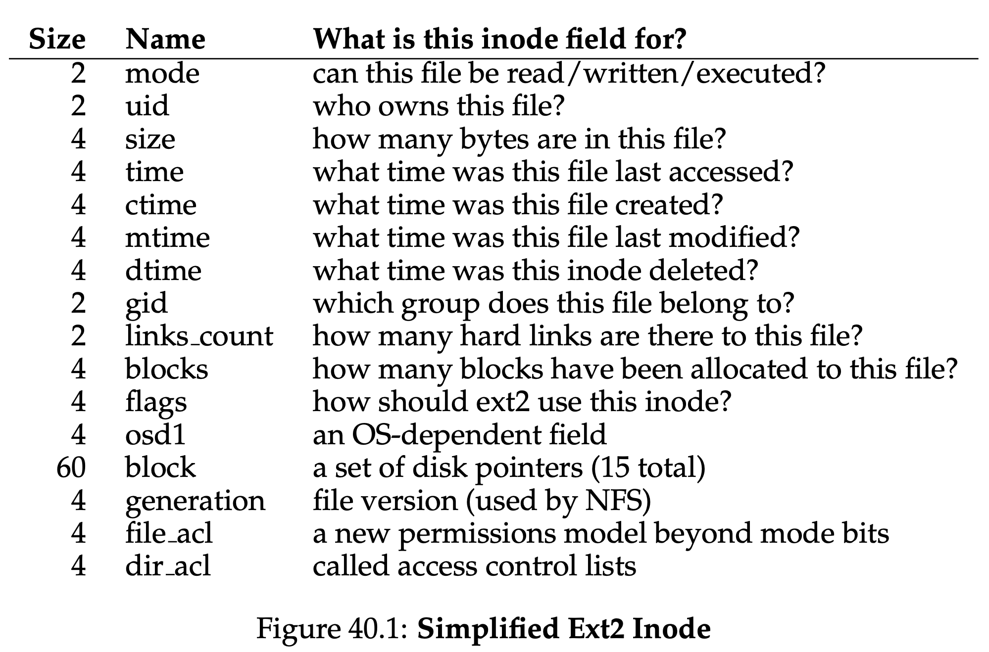
One of the most important decisions in the design of the inode is how it refers to where data blocks are. One simple approach would be to have one or more direct pointers(disk addresses) inside the inode; each pointer refers to one disk block that belongs to the file. Such an approach is limited, if you want to have a file that is really big.
The Multi-Level Index
To support bigger files, file system designers have had to introduce different structures within inodes. One common idea is to have a special pointer known as an indirect pointer. Instead of pointing to a block that contains user data, it points to a block that contains more pointers, each of which point to user data. Thus, an inode may have some fixed number of direct pointers, and a single indirect pointer. If a file grows large enough, an indirect block is allocated(from the data-block region of the disk), and the inode’s slot for an indirect pointer is set to point to it. Not surprisingly, in such an approach, you might want to support even larger files. To do so, just add another pointer to the inode: the double indirect pointer. This pointer refers to a block that contains pointers to indirect blocks, each of which contain pointers to data blocks.
Many researchers have studied file systems and how they are used, and virtually every time they find certain “truths” that hold across the decades. One such finding is that most files are small. This imbalanced design reflects such a reality; if most files are indeed small, it makes sense to optimize for this case.
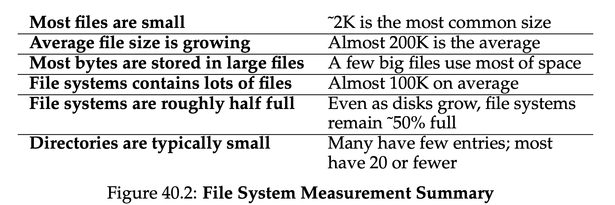
40.4 Directory Organization
In vsfs, directories have a simple organization; a directory basically just contains a list of(entry name, inode number) pair. For each file or directory in a given directory, there is a string and a number in the data block(s) of the directory.
You might be wondering where exactly directories are stored. Often, file systems treat directories as a special type of file. Thus, a directory has an inode, somewhere in the inode table(with the type field of the inode marked as “directory instead of “regular file”). The directory has data blocks pointed to by the inode; these data blocks live in the data block region of our simply file system. Our on-disk structure thus remains unchanged.
40.5 Free Space Management
A file system must track which inodes and data blocks are free, and which are not, so that when a new file or directory is allocated, it can find space for it.
40.6 Access Paths: Reading and Writing
Reading A File From Disk
A depiction of this entire process is found in Figure 40.3; time increases downward in the figure. In the figure, the open causes numerous reads to take place in order to finally locate the inode of the file. Afterwards, reading each block requires the file system to first consult the inode, then read the block, and then update the inode’s last-accessed-time field with a write.
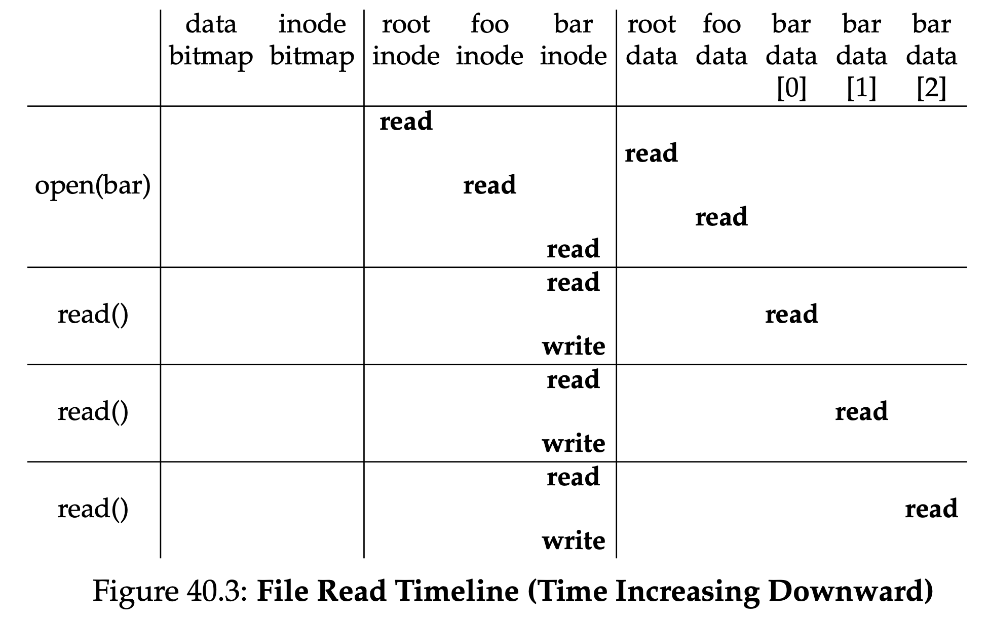
Writing A File To Disk
When writing out a new file, each write out only has to write data to disk but has to first decide which block to allocate to the file and thus update other structures of the disk accordingly(e.g., the data bitmap and inode). Thus, each write to a file logically generates five I/Os: one to read the data bitmap(which is the updated to mark the newly-allocated block as used), one to write the bitmap(to reflect its new state to disk), two more to read and then write the inode(which is updated with the new block’s location), and finally one to write the actual block itself.
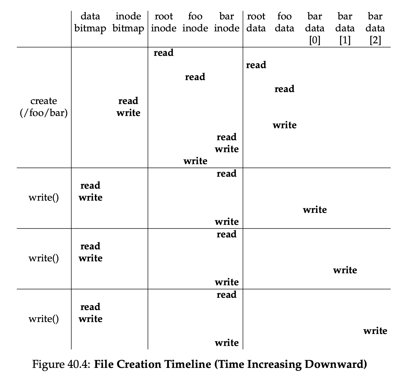
40.7 Caching and Buffering
As the examples above show, reading and writing files can be expensive, incurring many I/Os to the (slow) disk. To remedy what would clearly be a huge performance problem, most file systems aggressively use system memory(DRAM) to cache important blocks.
The first open may generate a lot of I/O traffic to read in directory inode and data, but subsquent file opens of that same file(or files in the same directory) will mostly hit in the cache and thus no I/O is needed. Whereas read I/O can be avoided altogether with a sufficiently large cache, write traffic has to go to disk in order to become persistent. Thus, a cache does not serve as the same kind of filter on write traffic that it does for reads. That said, writing buffer certainly has a number of performance benefit. First, by delaying writes, the file system can batch some updates into a smaller set of I/Os; second, by buffering a number of writes in memory, the system can then schedule the subsequent I/Os and thus increase performance. Finally, some writes are avoided altogether by delaying them; for example, if an application creates a file and then deletes it, delaying the writes to reflect the file creation to disk avoids them entirely. In this case, laziness(in writing blocks to disk) is a virtue.
For the reasons above, most modern file systems buffer writes in memory for anywhere between five and thirty seconds, representing yet another trade-off: if the system crashes before the updates have been propagated to disk, the updates are lost; however, by keeping writes in memory longer, performance can be improved by batching, scheduling, and even avoiding writes.
41 Locality and The Fast File System
41.1 The Problem: Poor Performance
The main issue was that the old UNIX file system treated the disk like it was a random-access memory; data was spread all over the place without regard to the fact that the medium holding the data was a disk, and thus had real and expensive positioning costs. For example, the data blocks of a file were often very far away from its inode, thus inducing an expensive seek whenever one first read the inode and then the data blocks of a file.
41.2 FFS:Disk Awareness Is The Solution
41.3 Organizing Structure: The Cylinder Group
FFS divides the disk into a number of cylinder groups. A single cylinder is a set of tracks on different surfaces of a hard drive that are the same distance from the center of the drive; it is called a cylinder because of its clear resemblance to the so-called geometrical shape. FFS aggregates N consecutive cylinders into a group, and thus the entire disk can thus be viewed as a collection of cylinder groups.
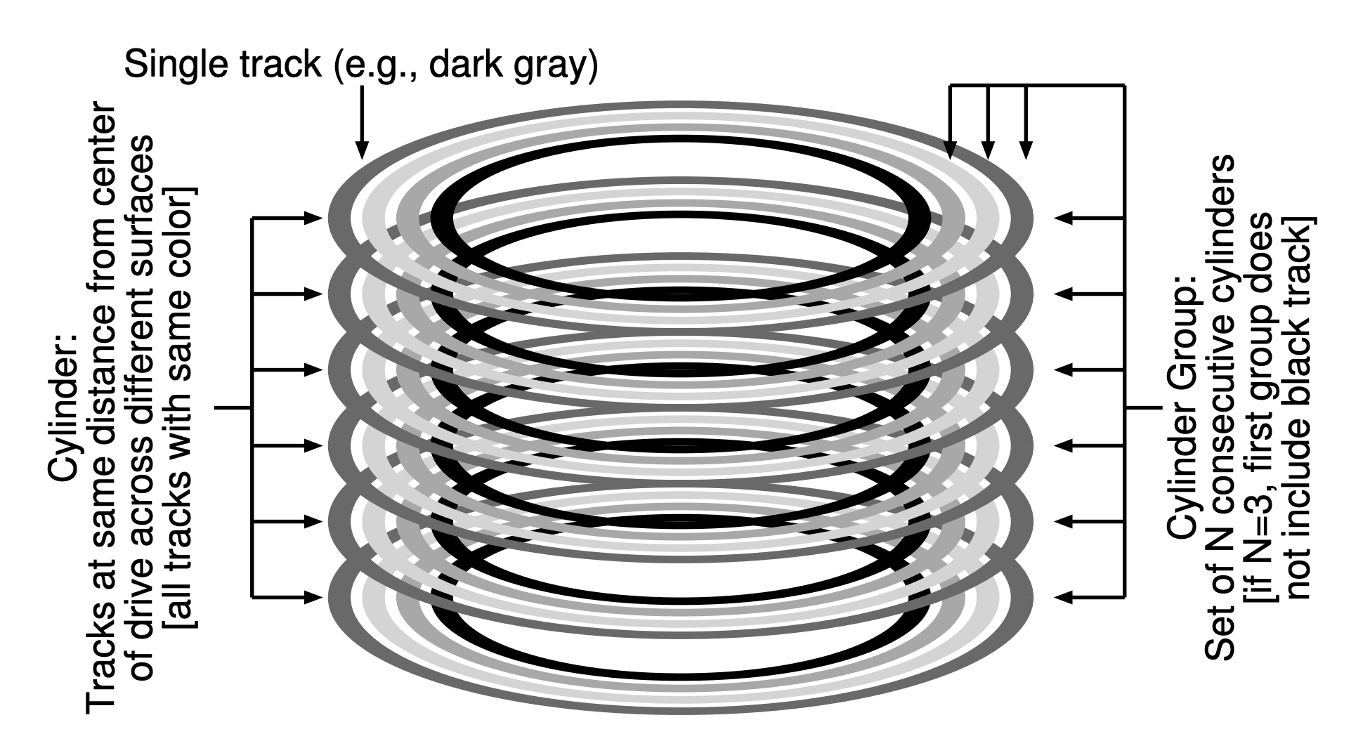
Whether you call them cylinder groups or block groups, these groups are the central mechanism that FFS uses to improve performance. Critically, by placing two files within the same group, FFS can ensure that accessing one after the other will not result in long seeks across the disk.
FFS keeps a copy of the super block(s) in each group for reliability reasons. The super block is needed to mount the file system; by keeping mulitple copies, if one copy becomes corrupt, you can still mount and access the file system by using a working replica. Within each group, FFS needs to track whether the inodes and data blocks of the group are allocated. A per-group inode bitmap(ib) and data bitmap(db) serve this role for inodes and data blocks in each group. Bitmaps are an excellent way to manage free space in a file system because it is easy to find a large chunk of free space and allcate it to a file, perhaps avoiding some of the fragmentation problems of the free list in the old file system. Most of each cylinder group, as usual, is comprised of data blocks.
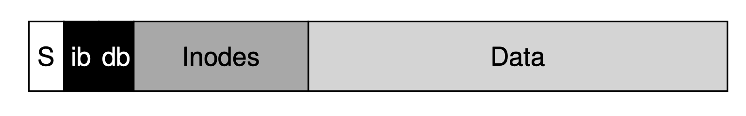
41.4 Policies: How To Allocate Files and Directories
The fist is the placement of directories. FFS employs a simple approach: find the cylinder group with a low number of allocated directories(to balance directories across groups) and a high number of free inodes(to subsequently be able to allocate a bunch of files), and put the directory data and inode in that group.
For files, FFS does two things. First, it makes sure to allocate the data blocks of a file in the same group as its inode, thus preventing long seeks between inode and data. Second, it places all files that are in the same directory in the cylinder group of the directory they are in.
41.6 The Large-File Exception
For large files, FFS does the following. After some number of blocks are allocated into the first block group, FFS places the next “large” chunk of the file in another block group. Then, the next chunk of the file is placed in yet another different block group, and so on.
Without the large-file exception, a single large file would place all of its blocks into one part of the disk. As you can see in the picture, /a fills up most of the data blocks in Group 0, whereas other groups remain empty. If some other files are now created in the root directory(/), there is not much room for their data in the group.
With the large-file exception,FFS instead spreads the file spread across groups,and the resulting utilization within any one group is not too high:
Spreading blocks of a file across the disk will hurt performance, particularly in the relatively common case of sequential file access. Specifically, if the chunk size is large enough, the file system will spend most of its time transferring data from disk and just a little time seeking between chunks of the block.
FFS took a simple approach to spread large files, based on the structure of the inode itself. The first twelve direct blocks were placed in the same group as the inode; each subsequent indirect block, and all the blocks it pointed to, was placed in a different group.
Note that the trend in disk drives is that transfer rate improves fairly rapidly, as disk manufactures are good at cramming more bits into the same surface, but the mechanical aspects of drives related to seeks(disk arm speed and the rate of rotation) improve rather slowly. The implication is that over time, mechanical costs become relatively more expensive, and thus, to amortize said costs, you have to transfer more data between seeks.
42 Crash Consistency:FSCK and Journaling
42.1 A Detailed Example
You can see that a single inode is allocated(inode number 2), which is marked in the inode bitmap, and a single allocated data block(data block 4), also marked in the data bitmap.
owner : remzi
permissions : read-write
size : 1
pointer : 4
pointer : null
pointer : null
pointer : null
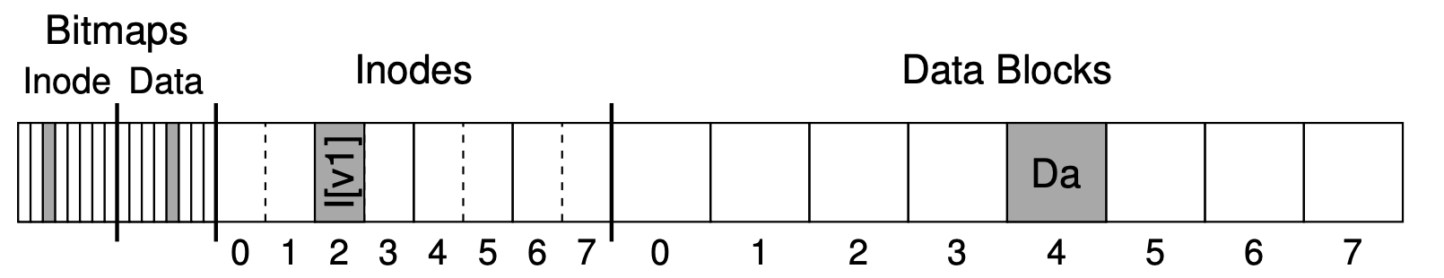
When we append to the file, we are adding a new data block to it, and thus must update three on-disk structures: the inode(which must point to the new block and record the new larger size due to the append), the new data block Db, and a new version of the data bitmap to indicate that the new data block has been allocated.
owner : remzi
permissions : read-write
size : 2
pointer : 4
pointer : 5
pointer : null
pointer : null
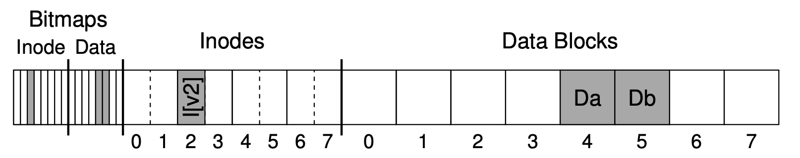
To achive this transition, the file system must perform three separate writes to the disk, one each for the inode, bitmap, and data block. Note that these writes usually don’t happen immediately when the user issues a write() system call; rather, the dirty inode, bitmap, and new data will sit in main memory(in the page cache or buffer cache) for some time first; then, when the file system finally decides to write them to disk(after say 5 seconds or 30 seconds), the file system will issue the requisite write requests to the disk. Unfortunately, a crash may occur and thus interfere with these updates to the disk. In particular, if a crash happens after one or two of these writes have taken place, but not all there,the file system could be left in a funny state.
Crash Scenarios
- Just the data block is written to disk.
- Just the update inode is written to disk.
- Just the updated bitmap is written to disk.
- The inode and bitmap are written to disk, but not data.
- The inode and the data block are written, but not the bitmap.
- The bitmap and data block are written, but not the inode.
The Crash Consistency Problem
We can have inconsistency in file system data structures; we can have space leaks; we can return garbage data to a user.
42.2 Solution #1: The File System Checker
Early file systems took a simple approach to crash consistency. Basically, they decided to let inconsistencies happen and then fix them later(when rebooting). A classic example of this lazy approach is found in a tool that does this: fsck. fsck is a UNIX tool for finding such inconsistencies and repairing them; similar tools to check and repair a disk partition exist on different systems. Note that such an approach can’t fix all problems; consider, for example, the case above where the file system looks consistent but the inode points to garbage data. The only real goal is to make sure the file system metadata is internally consistent.
Building a working fsck requires intricate knowledge of the file system; making sure such a piece of code works correctly in all cases can be challenging. However, fsck(and similar approaches) have a bigger and perhaps more fundamental problem: they are too slow. With a very large disk volume, scanning the entire disk to find all the allocated blocks and read the entire directory tree may take many minutes or hours. Performance of fsck, as disks grew in capacity and RAIDs grew in popularity, became prohibitive.
42.3 Solution #2: Journaling(or Write-Ahead Logging)
Probably the most popular solution to the consistent update problem is to steal an idea from the world of database management systems. That idea, known as write-ahead logging, was invented to address exactly this type of problem.
The basic idea is as follow. When updating the disk, before overwriting the structures in place, first write down a little note(somewhere else on the disk, in a well-known location) describing what you are about to do. Writing this note is the “write ahead” part, and we write it to a structure that we organize as a “log”; hence, write-ahead logging. By writing the note to disk, you are guaranteeing that if a crash takes places during the update(overwrite) of the structures you are updating, you can go back and look at the note you made and try again; thus, you will know exactly what to fix(and how to fix it) after a crash, instead of having to scan the entire disk. By design, journaling thus adds a bit of work during updates to greatly reduce the amount of work required during recovery.
We’ll now describe how Linux ext3, a popular journaling file system, incorporates journaling into the file system. Most of the on-disk structures are identical to Linux ext2. An ext2 file system(without journaling) looks like this:
Assuming the journal is placed within the same file system image, an ext3 file system with a journal looks like this:
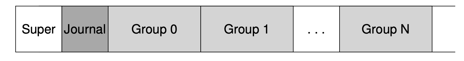
Data Journaling
Say we have our canonical update, where we wish to write the inode, bitmap, and data block to disk. Before writing them to their final disk locations, we are now first going to write them to the log(a.k.a. journal). This is what this will look like in the log:
The transaction begin(TxB) tells us about this update, including information about the pending update to the file system, and some kind of transaction identifier(TID). The middle three blocks just contain the exact contents of the blocks themselves; this is known as physical logging as we are putting the exact physical contents of the update in the journal. The final block(TxE) is a marker of the end of this transaction, and will also contain the TID. Once this transaction is safely on disk, we are ready to overwrite the old structures in the file system; this process is called checkpointing. Thus, to checkpoint the file system, we issue the write inode, bitmap, and data block to their disk locations as seen above; if these writes complete successfully, we have successfully checkpointed the file system and are basically done.
Things get a little tricker when a crash occurs during the writes to the journal. Here, we are trying to write the set of blocks in the transaction to disk. One simple way to do this would be to issue each one at a time, waiting for each to complete, and then issuing the next. However, this is slow. Ideally, we’d like to issue all five block writes at once, as this would turn five writes into a single sequential write and thus be faster. However, this is unsafe, for the following reason: given such a big write, the disk internally may perform scheduling and complete small piece of the big write in any order. Thus, the disk internally may write TxB, inode, bitmap, and TxE and only later write data block. Unforunately, if the disk loses power between them, this is what ends up on disk:
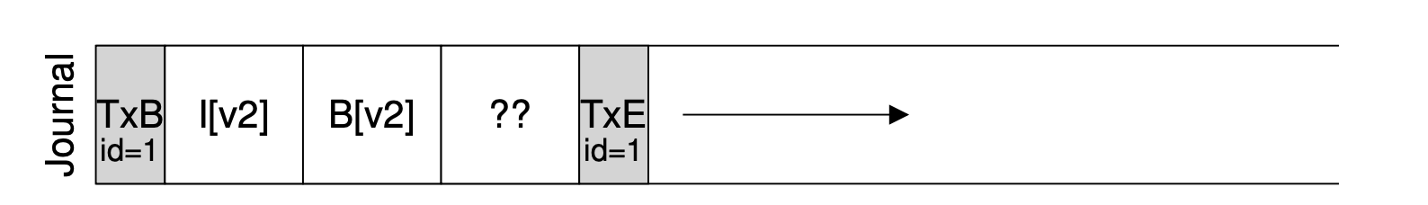
To avoid this problem, the file system issues the transactional write in two steps. First, it writes all blocks except the TxE block to the journal, issuing these writes all at once. When these writes complete, the journal will look something like this:
When those writes completes, the file system issue the write of the TxE block, thus leaving the journal in this final, safe state:
An important aspect of this process is the atomicity guarantee provided by the disk. It turns out that the disk guarantees that any 512-byte write will either happen or not(and never be half-written); thus, to make sure the write of TxE is atomic, one should make it a single 512-byte block.
Revoery
If the crash happens before the transaction is written safely to the log, then our job is easy: the pending update is simply skipped. If the crash the checkpoint is complete, the file system can recover the update as follows. When the system boots, the file system recovery process will scan the log and look for transactions that have committed to the disk; there transactions are thus replayed(in order), with the file system again atttempting to write out the blocks in the transaction to their final on-disk location. This form of logging is one of the simplest forms there is, and is called redo logging. By recovering the committed transactions in the journal, the file system ensures that the on-disk structures are consistent, and thus can proceed by mounting the file system and readying itself for new requests.
Batching Log Updates
Some file systems do not commit each update to disk one at a time(e.g., Linux ext3); rather, one can buffer all updates into a global transaction. In our example above, when the two files are created, the file system just marks the in-memory inode bitmap, inodes of the files, directory data, and directory inode as dirty, and adds them to the list of blocks that form the current transaction. When it is finally time to write these blocks to disk(say, after a timeout of 5 seconds), this single global transaction is committed containting all of the updates described above. Thus, by buffering updates, a file system can avoid excessive write traffic to disk in many cases.
Making The Log Finite
Two problems arise when the log becomes full. The first is simpler, but less critical: the larger the log, the longer recovery will take, as the recovery process must replay all the transactions within the log(in order) to recover. The second is more of an issue: when the log is full(or nearly full), no further transactions can be committed to the disk, thus making the file system “less than useful”(i.e., useless). To address these problems, journaling file systems treat the log as a circular data structure, re-using it over and over; this is why the journal is sometimes referred to as a circualr log.
Metadata Journaling
Because of the high cost of writing every data block to disk twice, people have tried a few different things in order to speed up performance. For example, the mode of journaling we described above is often called data journaling(as in Linux ext3), as it journals all user data. A simpler form of journaling is sometimes called ordered journaling(or just metadata journaling), and it is nearly the same, except that user data is not written to the journal. Thus, when performing the same update as above, the following information would be written to the journal.
The data block, previously written to the log, would instead be written to the file system proper, avoiding the extra write; given that most I/O traffic to the disk is data, not writing data twice substantially reduces the I/O load of journaling.
The update consists of three blocks: inode, bitmap and data block, some file systems(e.g., Linux ext3) write data blocks(of regular files) to the disk first, before related metadata is written to disk.
- Data write: Write data to final location; wait for completion.
- Journal metadata write: Write the begin block and metadata to the log; wait for writes to complete.
- Journal commit: Write the transaction commit block(containing TxE) to the log; wait for the write to complete; the transaction(including data) is now committed.
- Checkpoint metadata: Write the contents of the metadata update to their final locations within the file system.
- Free: Later, mark the transaction free in journal superblock. Finally, note that forcing the data write to complete(Step 1) before issuing writes to the journal(Step 2) is not required for correctness, as indicated in the protocol above. Specifically, it would be fine to concurrently issue writes to data, the transaction-begin block, and journaled metadata; the only real requirement is that Step 1 and 2 complete before the issuing of the journal commit block(Step 3).
By forcing the data write first, a file system can guarantee that a pointer will never point to garbage. Indeed, this rule of “write the pointed-to object before the object that points to it” is at the core of crash consistency, and is exploited even further by other crash consistency schemes.
43 Log-structured File Systems
When writing to disk, LFS first buffers all updates(including metadata!)in an in-memory segment; when the segment is full, it is written to disk in one long, sequential transfer to an unused part of the disk. LFS never overwrite existing data, but rather always writes segments to free locations. Because segmetns are large, the disk(or RAID) is used efficiently, and performance of the file system approaches its zenith.
43.1 Writing To Disk Sequentially
This basic idea, of simply writing all updates(such as data blocks, inode, etc.) to the disk sequentially, sits at the heart of LFS.
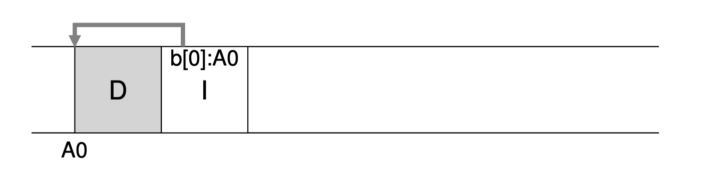
43.2 Writing Sequentially And Effectively
Before writing to the disk, LFS keeps track of updates in memory; when it has received a sufficient number of updates, it writes them to disk all at once, thus ensuring effcient use of the disk. The large chunk of updates LFS writes at one time is referred to by the name of segment. When writing to disk, LFS buffers updates in an in-memory segment, and then writes the segment all at once to the disk. As long as the segment is large enough, these writes will be efficient.
43.4 Problem: Finding Inodes
In LFS, finding inodes is more difficult. We’ve managed to scatter the inodes all throughout the disk! Worse, we never overwrite in place, and thus the latest version of an inode(i.e., the one we want) keeps moving.
43.5 Solution Through Indirection: The Inode Map
The imap is a structure that takes an inode number as input and produces the disk address of the most recent version of the inode. Any time an inode is written to disk, the imap is updated with its new location.
LFS places chunks of the inode map right next to where it is writing all of the other new information.
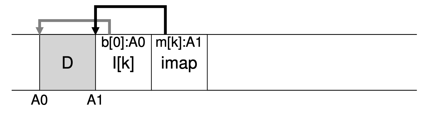
43.6 Completing The Solution: The Checkpoint Region
LFS has just such a fixed place on disk for this, known as the checkpoint region(CR). The checkpoint region contains pointers to the latest piece of the inode map, and thus the inode map piece can be found by reading the CR first. Note the checkpoint region is only updated periodically, and thus performance is not ill-affected. Thus, the overall structure of the on-disk layout contains a checkpoint region; the inode map pieces each contain addresses of the inodes; the inodes point to files(and directories) just like typical UNIX file system.
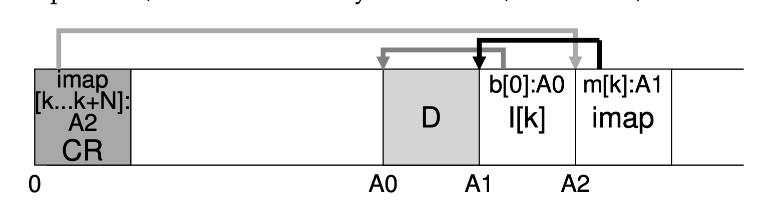
43.7 Reading A File From Disk: A Recap
The first on-disk data structure we must read is the checkpoint region. The checkpoint region contains pointers to the entire inode map, and thus LFS then reads in the entire inode map and caches it in memory. After this point, when given an inode number of a file, LFS simply looks up the inode-number to inode-disk-address mapping in the imap, and reads in the most recent version of the inode.
43.8 What About Directories?
When creating a file on disk, LFS must both write a new inode, some data, as well as the directory data and its inode that refer to this file. Remember that LFS will do so sequentially on the disk(after buffering the updates for some time).
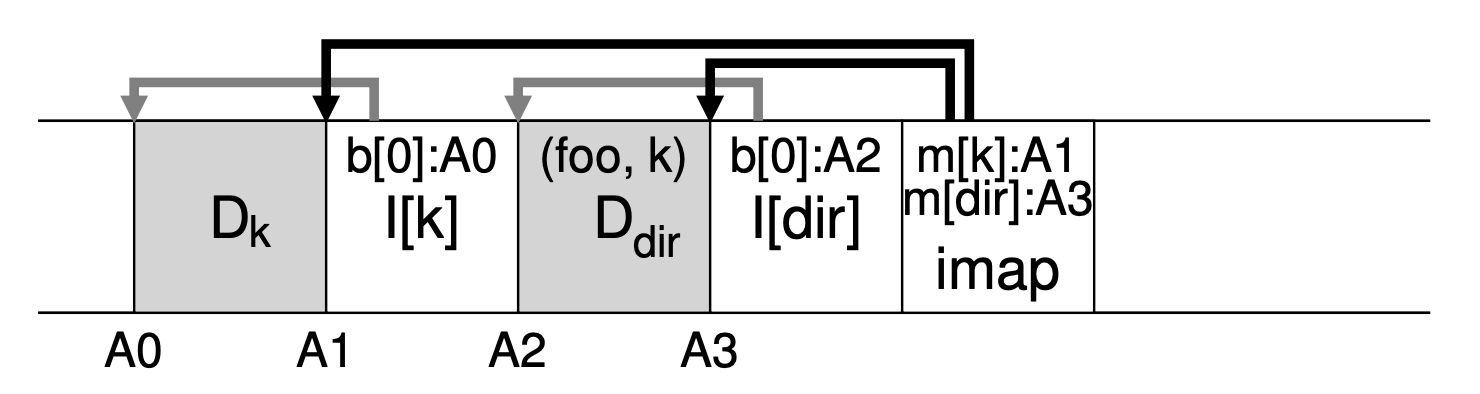
43.9 A New Problem: Garbage Collection
LFS instead keeps only the latest live version of a file; thus(in the background), LFS must periodically find these old dead versions of file data, inodes, and other structures, and clean them; cleaning should thus make blocks on disk free again for use in subsequent writes.
Periodically, the LFS cleaner reads in a number of old(partially-used) segments, determines which blocks are live within these segment, and then write out a new set of segments which just the live blocks within them, freeing up the old ones for writing.
43.10 Determining Block Liveness
For a block D located on disk at address A, look in the segment summary block and find its inode number N and offset T. Next, look in the imap to find where N lives and read N from disk. Finally, using the offset T, look in the inode to see where the inode thinks the Tth block of this file is on disk. If it points exactly to disk address A, LFS can conclude that the block D is live. If it points anywhere else, LFS can conclude that D is not in use and thus know that this version is no longer needed.
44 Flash-based SSDs
44.1 Storing a Single Bit
Flash chips are designed to store one or more bits in a single transistor; the level of charge trapped within the transistor is mapped to a binary value.
44.2 From Bits to Banks/Planes
Flash chips are organized into banks or planes which consist of a large number of cells.
A bank is accessed in two different sized units: blocks(sometimes called erase blocks), which are typically of size 128 KB or 256 KB, and pages, which are a few KB in size(e.g., 4KB). Within each bank there are a large number of blocks; within each block, there are a large number of pages.
The most important(and weird) thing you will learn is that to write to a page within a block, you first have to erase the entire block.
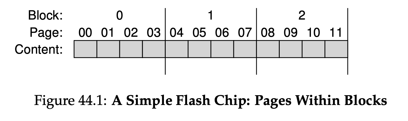
44.3 Basic Flash Operations
The read command is used to read a page from the flash; erase and program are used in tandom to write.
- Read(a page): A client of the flash chip can read any page, simply by specifying the read command and appropriate page number to the device. Being able to access any location uniformly quickly means the device is a random access device.
- Erase(a block): Before writing to a page within a flash, the nature of the device requires that you first earse the entire block the page lies within. Erase, importantly, destroys the contents of the block(by setting each bit to the value 1); therefore, you must be sure that any data you care about in the block has been copied elsewhere before executing the erase.
- Program(a page): Once a block has been erased, the program command can be used to change some of the 1’s within a page to 0’s, and write the desired contents of a page to the flash.
Once a page has been programmed, the only way to change its contents is to erase the entire block within which the page resides.
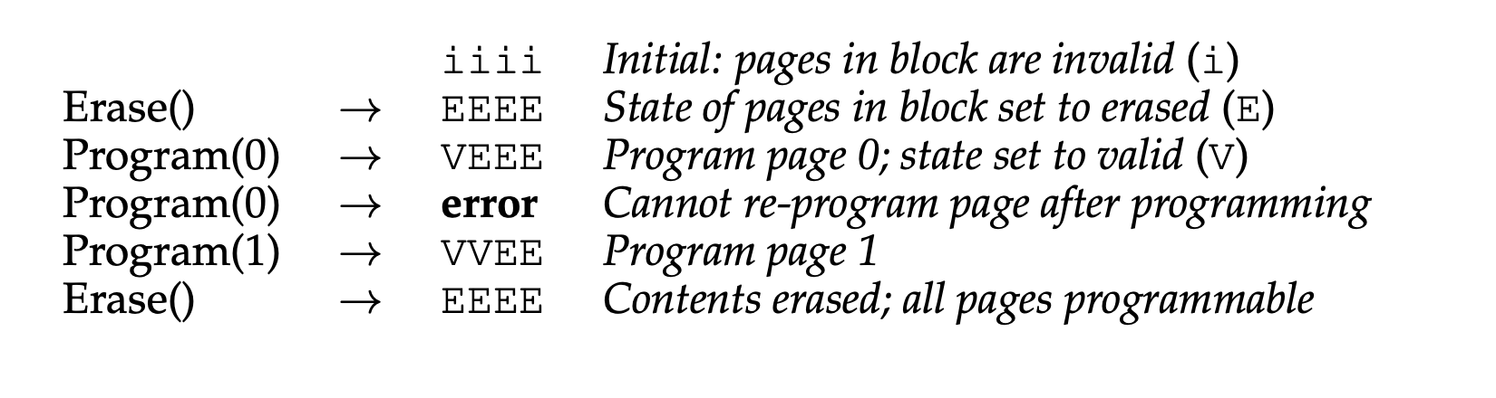
Frequent repetitions of this program/erase cycle can lead to the biggest reliability problem flash chips have: wear out.
44.4 Flash Performance And Reliability
The primary concern is wear out; when a flash block is erased and programmed, it slowly accrues a little bit of extra charge. Over time, as that extra charge builds up, it becomes increasingly difficult to differentiate between a 0 and a 1. One other reliability problem within flash chips is known as disturbance. When accessing a particular page within a flash, it is possible that some bits get flipped in neighboring page; such bit flips are known as read disturbs or program disturbs.
44.5 From Raw Flash to Flash-Based SSDs
Internally, an SSD consists of some number of flash chips(for persistent storage). An SSD also contains some amount of volatile(i.e., non-persistent) memory; such memory is useful for caching and buffering of data as well as for mapping tables. Finally, an SSD contains control logic to orchestrate device opertaion.
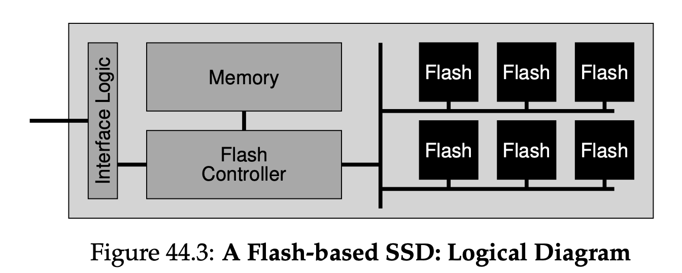
The flash translation layer(FTL) should try to spread writes across the blocks of the flash as evenly as possible, ensuring that all of the blocks of the device wear out at roughly the same time.
To minimize such disturbance, FTLs will commonly program pages within an erased block in order, from low page to high page.
45 Data Integrity and Protection
45.1 Disk Failure Modes
Latent-sector errors(LSEs) arise when a disk sector(or group of sectors) has been damaged in some way. There are also cases where a disk block becomes corrupt in a way not detectable by the disk itself.
If you really wish to build a reliable storage system, you must include machinery to detect and recover from both LSFs and block corruption.
45.2 Handling Latent Sector Errors
When a storage system tries to access a block, and the disk returns an error, the storage system should simply use whatever redundancy mechanism it has to return the correct data. In a mirrored RAID, for example, the system should access the alternate copy; in a RAID-4 or RAID-5 system based on parity, the system should reconstruct the block from the other blocks in the parity group.
45.3 Detection Corruption: The Checksum
The primary mechanism used by modern storage systems to preserve data integrity is called the checksum. A checksum is simply the result of a function that takes a chunk of data as input and computes a function over said data, producing a small summary of the contents of the data. The goal of such a computation is to enable a system to detect if data has somehow been corrupted or altered by storing the checksum with the data and then confirming upon later access that the data’s current checksum matches the original storage value.
45.4 Using Checksums
When reading a block D, the client also reads its checksum from disk $C_{s}$(D),which we call the stored checksum. The client then computes the checksum over the retrieved block D, which we call the computed checksum $C_{c}$(D). At this point, the client compares the stored and computed checksums; if they are equal, the data has likely not been corrupted, and thus can be safely returned to the user.
45.5 A New Problem: Misdirected Writes
This arises in disk and RAID controllers which write the data to disk correctly, except in the wrong location. In this case, adding a physical identifier(physical ID) is quite helpful. If the stored information now contains the checksum C(D) and both the disk and sector numbers of the block, it is easy for the client to determine whether the correct information resides within a particular locale.
45.6 One Last Problem: Lost Writes
Lost writes occurs when the device informs the upper layer that a write has completed but in fact it never is persisted; thus, what remains is the old contents of the block rather than the updated new contents.
One classic approach is to perform a write verify or read-after-write; by immediately reading back the data after a write, a system can ensure that the data indeed reached the disk surface. This approach, however, is quite slow, doubling the number of I/Os needed to complete a write.
45.7 Scrubbing
By periodically reading through every block of the system, and checking whether checksums are still valid, the disk system can reduce the chances that all copies of a certain data item become corrupted. Typical systems schedule scans on a nightly or weekly basis.
45.8 Overheads Of Checksumming
The first is on the disk itself; each stored checksum takes up room on the disk, which can no longer be used for user data. The second type of space overhead comes in the memory of the system. When accessing data, there must now be room in memory for the checksums as well as the data itself.
While space overheads are small, the time overheads induced by checksumming can be quite noticeable. One approach to reducing CPU overheads, employed by many system that use checksums(including network stacks), is to combine data copying and checksumming into one streamlined activity.
48 Distributed Systems
48.1 Communication Basic
The central tenet of modern networking is that communication is fundamentally unreliable. Whether in the wide-area Internet, or a local-area high-speed network such as Infiniband, packets are regularly lost, corrupted, or otherwise do not reach their destination.
48.2 Unreliable Communication Layers
One excellent example of such an unreliable layer is found in the UDP/IP networking stack available today on virtually all modern systems. If you use it, you will encounter situations where packets get lost(dropped) and thus do not reach their destination; the sender is never thus informed of the loss. However, that does not mean that UDP does not guard against any failures at all. For example, UDP includes a checksum to detect some forms of packet corruption.
48.3 Reliable Communication Layers
The technique that we will use is known as an acknowledgment, or ack for short. The sender sends a message to the receiver; the receiver then sends a short message back to acknowledge its receipt.
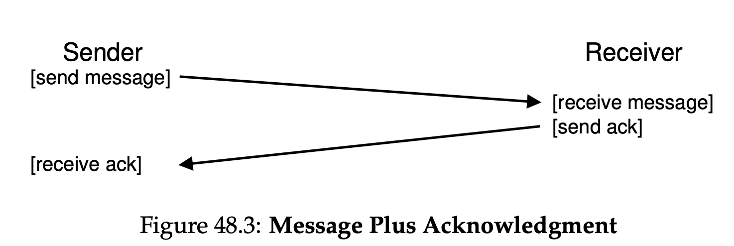
When we are aiming for a reliable message layer, we also usually want to guarantee that each message is received exactly once by the receiver. To enable the receiver to detect duplicate message transmission, the sender has to identify each message in some unique way, and the receiver needs some way to track whether it has already seen each message before. When the receiver sees a duplicate transmission, it simply acks the message, but(critically) does not pass the message to the application that receives the data. Thus, the sender receives the ack but the message is not received twice, preserving the exactly-once semantics mentioned above.
With a sequence counter, the sender and receiver agree upon a start value(e.g., 1) for a counter that each side will maintain. Whenever a message is sent, the current value of the counter is sent along with the message; this counter value(N) serves as an ID for the message. After the message is sent, the sender then increments the value(to N + 1). The receiver uses its counter value as the expected value for the ID of the incoming message from that sender. If the ID of a received message(N) matches the receiver’s counter(also N), it acks the message and passes it up to the application; in this case, the receiver concludes this is the first time this message has been received. The receiver then increments its counter(to N + 1),and waits for the next message.
The most commonly used reliable communication layer is known as TCP/IP, or just TCP for short.
49 Sun’s Network File System(NFS)
One of the first uses of distributed client/server computing was in the realm of distributed file systems. In such an enviroment, there are a number of client machines and one server(or a few); the server stores the data on its disk, and clients request data through well-formed protocol messages.
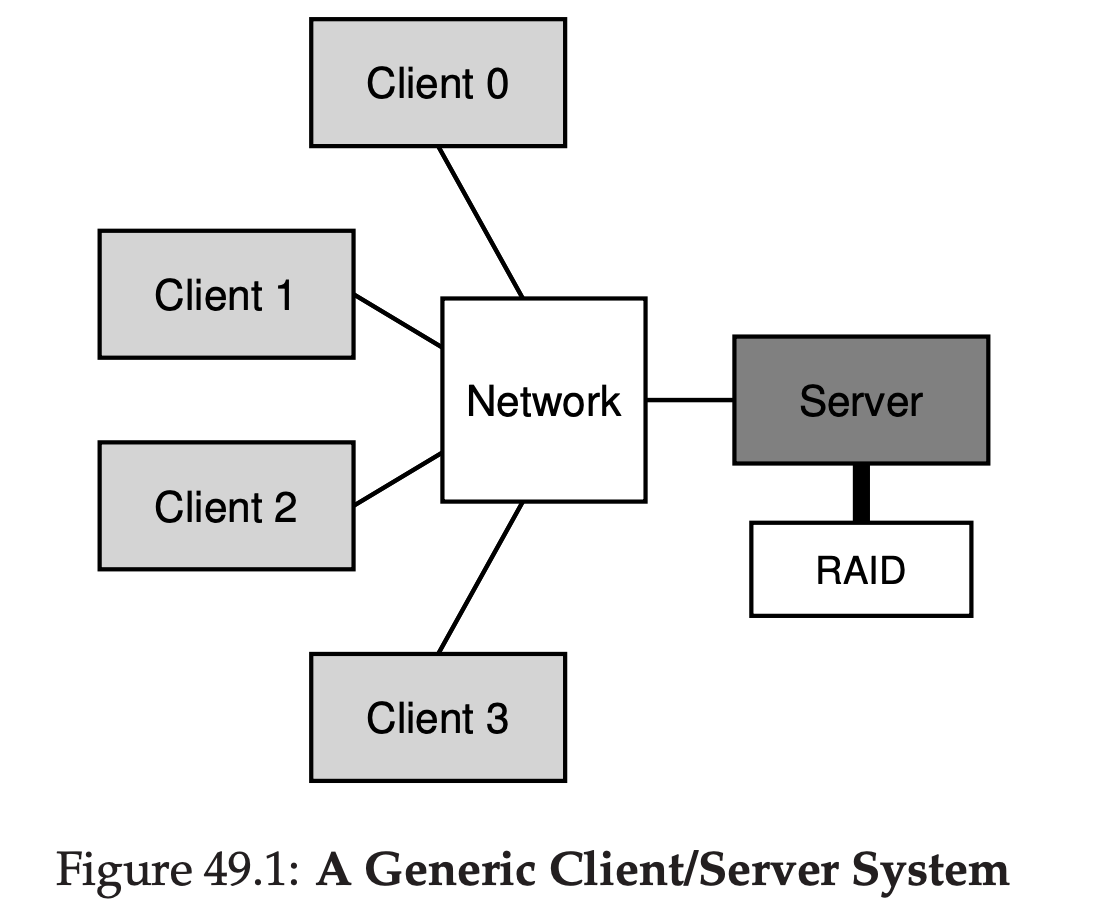
49.1 A Basic Distributed File System
On the client side, there are client applications which access files and directories through the client-side file system. A client application issues system calls to the client-side file system in order to access files which are stored on the server. The role of the client-side file system is to execute the actions needed to service those system calls. For example, if the client issues a read() request, the client-side file system may send a message to the server-side file system to read a particular block; the file server will then read the block from disk, and send a message back to the client with the requested data. The client-side file system will then copy the data into the user buffer supplied to the read() system call and thus the request will complete. Note that a subsequent read() of the same block on the client may be cached in client memory or on the client’s disk even; in the best such case, on network traffic need be generated.
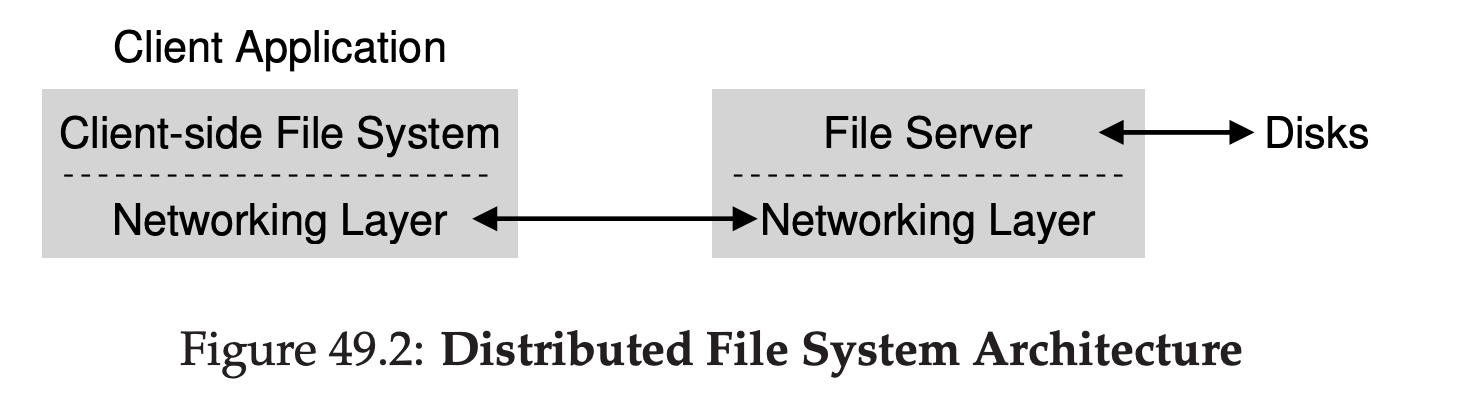
49.4 Key To Fast Crash Recovery: Statelessness
The server doesn’t track anything about what clients are doing; rather, the protocol is designed to deliver in each protocol request all the information that is needed in order to complete the request.
49.5 The NFSv2 Protocol
First, the LOOKUP protocol message is used to obtain a file handle, which is then subsequently used to access file data. The client passes a directory file handle and name of a file to look up, and the handle to that file(or directory) plus its attributes are pass ack to the client from the server.
49.6 From Protocol To Distributed File System
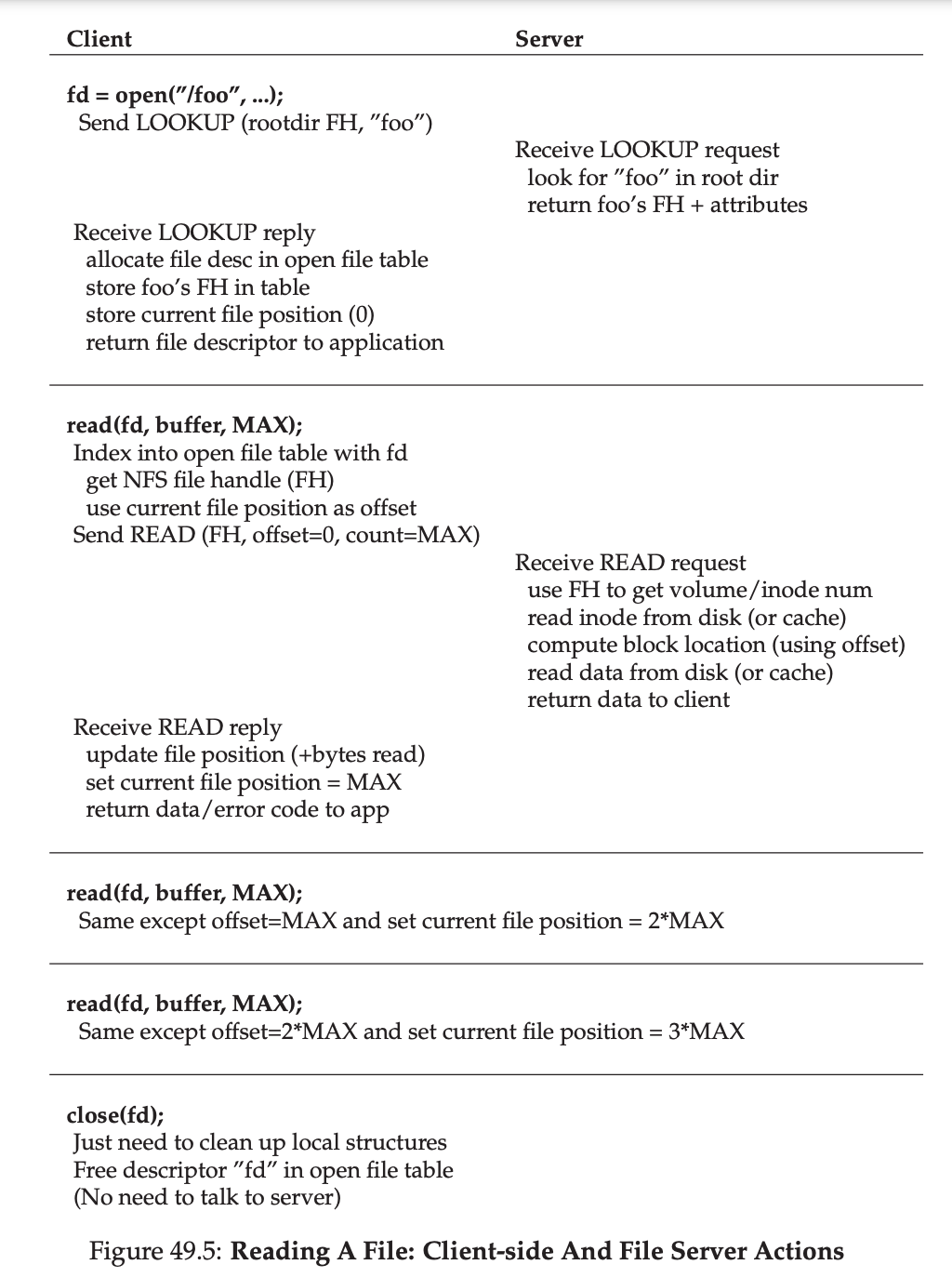
49.7 Handling Server Failure With Idempotent Operations
In NFSv2, a client handles all of these failures in a single, uniform, and elegent way: it simply retries the request. Specifically, after sending the request, the client sets a timer to go off after a specified time period. If a reply is received before the timer goes off, the timer is canceled and all is well. If, however, the timer goes off before any reply is received, the client assumes the request has not been processed and resends it. If the server replies, all is well and the client has neatly handled the problem.
The ability of the client to simply retry the request(regardless of what caused the failure)is due to an important property of most NFS requests: they are idempotent. More generally, any operation that just reads data is obviously idempotent. an operation that updates data must be more carefully considered to determine if it has this property.
The heart of the design of crash recovery in NFS is the idempotency of most common operations. LOOKUP and READ requests are trivially idempotent, as they only read information from the file server and do not update it. More interestingly, WRITE requests are also idempotent. If, for example, a WRITE fails, the client can simply retry it. The WRITE message contains the data, the count, and(importantly) the exact offset to write the data to. Thus, it can be repeated with the knowledge that the outcome of mulitple writes is the same as the outcome of a single one.
A small aside: some operations are hard to make idempotent. For example, when you try to make a directory that already exists, you are informed that the mkdir request has failed. Thus, in NFS, if the file server receives a MKDIR protocol message and executes it successfully but the reply is lost, the client may repeat it and encounter that failure when in fact the operation at first succeeded and then only failed on the retry. Thus, life is not perfect.
The NFS design philosophy covers most of the important cases, and overall makes the system design clean and simple with regards to failure. The best is the enemy of the good.
49.8 Improving Performance: Client-side Caching
The NFS client-side file system cache file data(and metadata) that it has read from the server in client memory. Thus, while the first access is expensive(i.e., it requires netowkr communication), subsequent accesses are serviced quite quickly out of client memory.
Adding cache into any sort of system with multiple client caches introduces a big and interesting challedge which we will refer to as the cache consistency problem.
49.9 The Cahce Consistency Problem
The first problem is that the client C2 may buffer its writes in its cache for a time before propagating them to the server; in this case, while F(v2) sits in C2’s memory, any access of F from another client(say C3) will fetch the old version of the file(F[v1]). Thus, by buffering writes at the client, other clients may get stale versions of the file, which may be undersirable; indeed, imagine the case where you log into machine C2, update F, and then log into C3 and try to read the file, only to get the old copy. Let’s call this aspect of the cache consistency problem update visibility. The second problem of cahce consistency is a stale cache; in this case, C2 has finally flushed its writes to the file server, and thus the server has the latest version(F[v2]). However, C1 still has F[v1] in its cache; if a program running on C1 reads file F, it will get a stale version F[v1] and not the most recent copy F[v2], which is(often) undesirable.
NFSv2 implementations solve these cache consistency problems in two ways. First, to address update visibility, clients implmement what is sometimes called flush-on-close(a.k.a., close-to-open) consistency semantics; specifically, the client flushes all updates(i.e., dirty pages in the cache) to the server. With flush-on-close consistency, NFS ensures that a subsequent open from another node will see the latest file version. Second, to address the stale-cache problem, NFSv2 clients first check to see whether a file has changed before using its cache contents. Specifically, before using a cache block, the client-side file system will issue a GETATTR request to the server to fetch the file’s attributes. The attributes, importantly, include information as to when the file was last modified on the server; if the time-of-modification is more recent than the time that the file was fetched into the client cache, the client invalidates the file, thus removing it from the client cache and ensuring that subsequent reads will go to the server and retrieve the latest version of the file. If, on the other hand, the client sees that it has the latest version of the file, it will go ahead and use the cached contents, thus increasing performance.
A client would still validate a file before accessing it, but most often would just look in attribute cache to fetch the attributes. The attributes for a particular file were placed in the cache when the file was first accessed, and then would timeout after a certain amount of time(say 3 seconds). Thus, during those three seconds, all file accesses would determine that it was OK to use the cached file and thus do so with no network communication with the server.
49.11 Implications On Server-Side Write Buffering
NFS servers must commit each write to stable storage before informing the client of success; doing so enables the client to detect server failure during a write, and thus retry until it finally succeeds. Writing performance can be the major bottleneck. One trick is to first put writes in a battery-backed memory, thus enabling to quickly reply to WRITE requests without fear of losing the data and without the cost of having to write to disk right away; the second trick is to use a file system design specifically designed to write to disk quickly when one finally needs to do so.
50 The Andrew File System(AFS)
50.1 AFS Version 1
One of the basic tenets of all versions of AFS is whole-file caching on the local disk of the client machine that is accessing a file. When you open() a file, the entire file(if it exists) is fetched from the server and stored in a file on your local disk. Subsequent application read() and write() operations are redirected to the loca file system where the file is stored; thus, these operations require no network communication and are fast. Finally, upon close(), the file(if it has been modified) is flushed back to the server.
50.4 AFS Version 2
A callback is simply a promise from the server to the client that the server will inform the client when a file that the client is caching has been modified. By adding this state to the system, the client no longer needs to contact the server to find out if a cached file is still valid. Rather, it assumes that the file is valid until the server tells it otherwise.
An FID in AFS consists of a volume identifier, a file identifier, and a “uniquifier”. Thus, instead of sending whole pathnames to the server and letting the server walk the pathname to find the desired file, the client would walk the pathname, one piece at a time, caching the results and thus hopefully reducing the load on the server.
50.5 Cache Consistency
Between different machines, AFS makes updates visible at the server and invalidates cached copies at the exact same time, which is when the updated file is closed. A client opens a file, and then writes to it. When it is finally closed, the new file is flushed to the server. At this point, the server then “breaks” callbacks for any clients with cached copies; the break is accomplished by contacting each client and informed it that the callback it has on the file is no longer valid. This step ensures that clients will no longer read stale copies of the file; subsequent opens on those clients will require a re-fetch of the new version of the file from the server( and will also serve to reestablish a callback on the new version of the file).
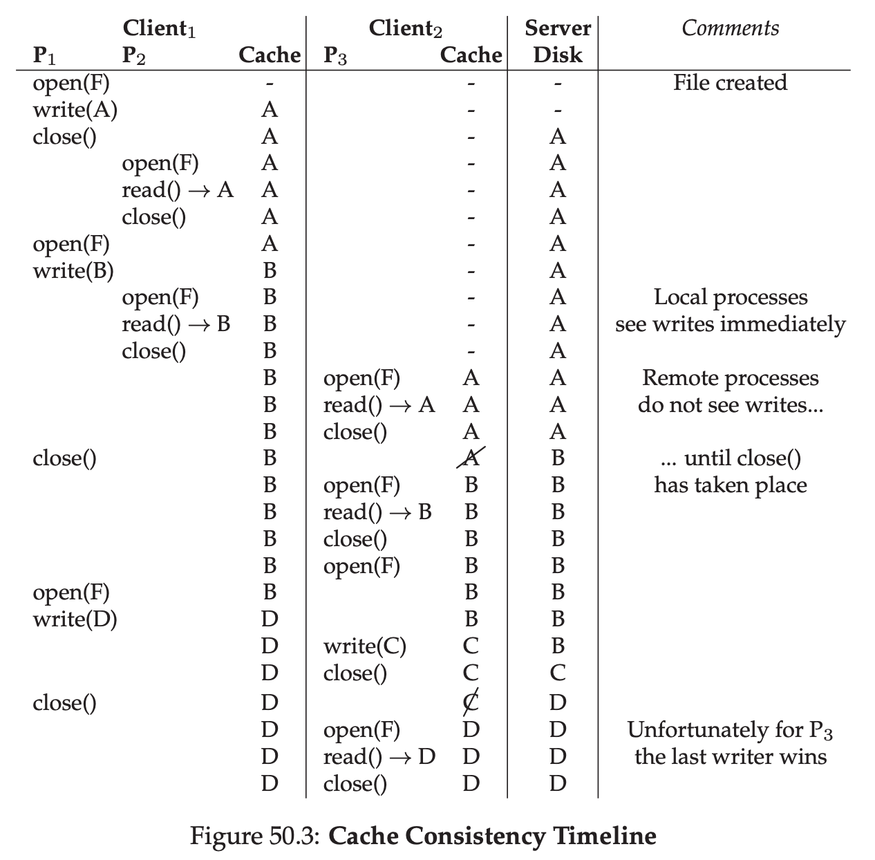
53 Introduction to Operating System Security
53.3 Security Goals and Policies
As a high conceptual level, they have defined three big security-related goals that are common to many systems: 1、 Confidentitality - If some piece of information is supported to be hidden from others, don’t allow them to find it out. 2、 Integrity - If some piece of information or component of a system is supposed to be in a particular state, don’t allow an adversary to change it. 3、Availability - If some information or service is supposed to be available for your own or other’s use, make sure an attacker cann’t prevent its use.
53.4 Designing Secure Systems
1、 Economy of mechanism - This basically means keep your system as small and simple as possible.
2、Fail-safe defaults - Default to security, not insecurity. 3、Complete mediation - This is a security term meaning that you should check if an action to be performed meets security policies every single time the action is taken. 4、Open design - Assume your adversary knows every detail of your design. If the system can achieve its security goals anyway, you’re in good shape. 5、Seperation of privilege - Require separate parties or credentials to perform critical actions. 6、Least privilege - Give a user or a process the minimum privileges required to perform the actions you wish to allow. 7、Least common mechanism - For different users or processes, use separate data structures or mechanisms to handle them. 8、Acceptability - A critical property not dear to the hearts of many programmers.
53.5 The Basic of OS Security
A lot of system security is going to be related to process handling.